Download

1 / 23
250 likes | 628 Views
2D Deformation and Creep Response of Articular Cartilage. By: Mikhail Yakhnis & Robert Zhang. Motivation. Articular cartilage transfers load between bones enables smooth motion along joints Cartilage has limited capacity for self repair

E N D
2D Deformation and Creep Response of Articular Cartilage By: Mikhail Yakhnis & Robert Zhang
Motivation • Articular cartilage • transfers load between bones • enables smooth motion along joints • Cartilage has limited capacity for self repair • Applications: biomaterials, prosthetics, biomedical devices http://nigelhartnett.onlinemedical.com.au/images/articular%20knee%20injury.jpg
Problem Description • Consider cartilage in an unconfined compression under constant load F • Analyze the 2D elastic deformation over time F Compression plate Articular Cartilage Frictionless Supports
Material Background • Cartilage often modeled as a viscoelastic material • Viscous and elastic by superposition • Elasticity and viscosity can be linear or nonlinear • Established models: Kelvin-Voigt, Maxwell, Standard-Linear Solid http://www.allsealsinc.com/allseals/Orings/maxwell.gif
Mathematical Model for Cartilage • We chose the Kelvin-Voigt model to focus on the creep response • The constitutive equation is Mechanical Analogue of Kelvin-Voigt Model http://en.wikipedia.org/wiki/File:Kelvin_Voigt_diagram.svg
Assumptions for Model • Conditions • Constant force Fnormal to boundary B3 • No gravity (body force) • 2D, plane stress* • Confined in y-direction along B1andB3 • Confined in x-direction along B4 • Properties • c = 0.1m; L = 0.125m • Constant cross-sectional area A • Isotropic elasticity* * L c F B3 B4 B2 y B1 x
Experimental Data • (Aggregate Modulus) Data Book on Mechanical Properties of Living Cells, Tissues, and Organs /. Tokyo ; New York : Springer, 1996. Print.
Derivation of Weak Form • By definition, stress • Strain can be rewritten as gradient of displacement u • Our constitutive equation (in strong form) becomes
Derivation of Weak Form (1) Take the gradient of the force equation (which equals zero) (2) Multiply by an arbitrary displacement (3) Integrate by parts to induce symmetry of and
Decoupling a Transient Problem • We can decouple the formulation and assume the time and spatial variations are separate where is a function of time only and basis function N is function of space • The weak differential equation rewritten in matrix form is Reddy, J. N.. "Time-Dependent Problems." An introduction to nonlinear finite element analysis. Oxford: Oxford University Press, 2004. . Print.
Displacement Equation for Creep Response • At each time step n • The equation for becomes
Modeling Creep in MATLAB • Changes in Preprocessor.m • Provide initial displacement • Define time step • Adjust boundary conditions • Changes in Assemble.m • Assemble the damping matrix [C] • Changes in NodalSoln.m • Add initial condition, damping, time inputs • Modify reaction force and displacement equations
Modeling Creep in MATLAB • Discussion: • MATLAB result converges toward experimental data farther away from initial time • 10% error at 6 seconds • MATLAB model reaches equilibrium faster than experimental data
Modeling Creep in ANSYS • A variety of models are available • Differences include suitability for primary and secondary creep • Usually of the form • Examples • Strain Hardening: • Time Hardening: ANSYS Advanced Nonlinear Materials: Lecture 3 – Rate Dependent Creep http://www.ansys-blog.com/wp-content/uploads/2012/06/Three-Types-of-Creep.png
Considerations for ANSYS Model • What experimental data is available to us? • Can we fit the experimental data to the model? • Can we use the built-in Mechanical APDL curve fitting procedure? • Is there more emphasis on primary creep or secondary creep? • Does the model satisfy our constitutive equation?
Parameters in the ANSYS Model • Experimental data provides aggregate modulus and Poisson’s ratio • Young’s Modulus can be derived from • The solution for time-dependent strain in the K-V model is • We can use the Modified Exponential Function in ANSYS where ; we can solve for and ANSYS Advanced Nonlinear Materials: Lecture 3 – Rate Dependent Creep
ANSYS Results – Creep Response Short Term Response – 30 Seconds Long Term Response – 3000 Seconds
Comparison of ANSYS and Experiment • Result: • Theoretical Model-Based ANSYS data tends to overshoot experimental data • Error is between 30% to 40% per data point • Experimental-based model performs better • Discussion: • Results demonstrate the limitations of ANSYS models • A combined primary-secondary model is ideal • Long term response in ANSYS is not accurate • Function models primary response Primary + Secondary Time Hardening
Sensitivity Analysis • Recall the creep model: • We varied each non-zero model constant by 50%* to perform a rudimentary sensitivity analysis: *The simulation did not converge at C2 +50% so C2 +10% was used instead
2D Deformation and Creep Response of Articular Cartilage By: DJ Mikey Mike & Big Rob Zhang Thank you for listening. Questions?