Download
1 / 20
350 likes | 1.15k Views
Chapter 2 Frequency Distributions and Graphs. Section 2-2. Organizing Data. Frequency distribution - is the organization of raw data in table form, using classes and frequencies.

E N D
Chapter 2 Frequency Distributions and Graphs Section 2-2 Organizing Data
Frequency distribution - is the organization of raw data in table form, using classes and frequencies. Categorical frequency distribution - is used for data that can be placed in specific categories, such as nominal- or ordinal-level data
Section 2-2 Exercise #7 A survey was taken on how much trust people place in the information they read on the Internet. Construct a categorical frequency distribution for the data. A = trust in everything they read, M = trust in most of what they read, H = trust in about half of what they read, S = trust in a small portion of what they read.
Constructing a Grouped Frequency Distribution Step 1 Determine the classes. • Find the highest and lowest value. • Find the range. • Select the number of classes desired. • Find the width by dividing the range by the number of classes and rounding up. • Select a starting point (usually the lowest value or any convenient number less • than the lowest value); add the width to get the lower limits. • Find the upper class limits. • Find the boundaries. Step 2 Tally the data. Step 3 Find the numerical frequencies from the tallies. Step 4 Find the cumulative frequencies.
Section 2-2 Exercise #11 The average quantitative GRE scores for the top 30 graduate schools of engineering are listed below. Construct a frequency distribution with six classes.
Section 2-2 Exercise #13 The ages of the signers of the Declaration of Independence are shown below (age is approximate since only the birth year appeared in the source, and one has been omitted since his birth year is unknown). Construct a frequency distribution for the data using seven classes.
Chapter 2 Frequency Distributions and Graphs Section 2-3 Histograms, Frequency Polygons, and Ogives
The three most commonly used graphs in research are as follows: 1. The histogram. 2. The frequency polygon. 3. The cumulative frequency graph, or ogive (pronounced o-jive).
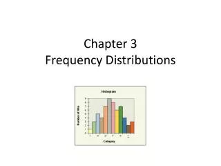
Histogram The histogram is a graph that displays the data by using contiguous vertical bars (unless the frequency of a class is 0) of various heights to represent the frequencies of the classes.
Frequency Polygon The frequency polygon is a graph that displays the data by using lines that connect points plotted for the frequencies at the midpoints of the classes. The frequencies are represented by the heights of the points.
Ogive The ogive is a graph that represents the cumulative frequencies for the classes in a frequency distribution.
Constructing Statistical Graphs Step 1 Draw and label the x and y axes. Step 2 Choose a suitable scale for the frequencies or cumulative frequencies, and label it on the y axis. Step 3 Represent the class boundaries for the histogram or ogive, or the midpoint for the frequency polygon, on the x axis. Step 4 Plot the points and then draw the bars or lines.
Class limits Frequency 90 – 98 6 99 – 107 22 108 – 116 43 117 – 125 28 126 – 134 9 Section 2-3 Exercise #1 For 108 randomly selected college applicants, the following frequency distribution for entrance exam scores was obtained. Construct a histogram, frequency polygon, and ogive for the data.
Section 2-3 Exercise #1 Applicants who score above 107 need not enroll in a summer developmental program. In this group, how many students do not have to enroll in the developmental program?
Section 2-3 Exercise #7 The air quality measured for selected cities in the United States for 1993 and 2002 are shown. The data are the number of days per year that the cities failed to meet acceptable standards. Construct a histogram for both years and see if there are any notable changes. If so, explain.
Section 2-3 Exercise #15 The number of calories per serving for selected ready - to - eat cereals is listed here. Construct a frequency distribution using seven classes. Draw a histogram, frequency polygon, and ogive for the data, using relative frequencies. Describe the shape of the histogram.
When the peak of a distribution is to the left and the data values taper off to the right, a distribution is said to be positively or right-skewed. See Figure 2–8(e). • When the data values are clustered to the right and taper off to the left, a distribution is said to be negatively or left-skewed. • Distributions with one peak, such as those shown in Figure 2–8(a), (e), and (f), are said to be unimodal. (The highest peak of a distribution indicates where the mode of the data values is. The mode is the data value that occurs more often than any other data value.) • When a distribution has two peaks of the same height, it is said to be bimodal. See Figure 2–8(g). • Finally, the graph shown in Figure 2–8(h) is a U-shaped distribution.