Download
1 / 84
840 likes | 846 Views
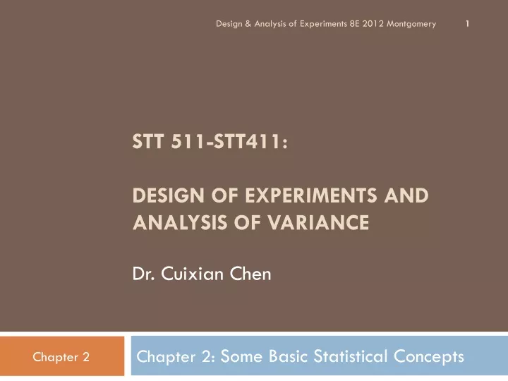
STT 511-STT411: DESIGN OF EXPERIMENTS AND ANALYSIS OF VARIANCE Dr. Cuixian Chen. Chapter 2: Some Basic Statistical Concepts. Review of STT215: Chapter 3. 3.1 Design Of Experiments (Outline of a randomized designs).

E N D
Design & Analysis of Experiments 8E 2012 Montgomery STT 511-STT411:DESIGN OF EXPERIMENTS AND ANALYSIS OF VARIANCEDr. Cuixian Chen Chapter 2: Some Basic Statistical Concepts
3.1 Design Of Experiments(Outline of a randomized designs) Completely randomized experimental designs: Individuals are randomly assigned to groups, then the groups are randomly assigned to treatments.
Example 3.13, page 179 What are the effects of repeated exposure to an advertising message (digital camera)? The answer may depend on the length of the ad and on how often it is repeated. Outline the design of this experiment with the following information. • Subjects: 150 Undergraduate students. • Two Factors: length of the commercial (30 seconds and 90 seconds – 2 levels) and repeat times (1, 3, or 5 times – 3 levels) • Response variables: their recall of the ad, their attitude toward the camera, and their intention to purchase it. (see page 187 for the diagram.) HWQ: 3.18, 3.30(b),3.32
3.1 Design Of Experiments (Block designs) In a block,orstratified, design, subjects are divided into groups, or blocks, prior to experiments to test hypotheses about differences between the groups. The blocking, or stratification, here is by gender (blocking factor). EX3.19 Ex: 3.17 (p182), 3.18 HWQ: 3.47(a,b), 3.126.
The most closely matched pair studies use identical twins. 3.1 Design Of Experiments (Matched pairs designs) Matched pairs: Choose pairs of subjects that are closely matched—e.g., same sex, height, weight, age, and race. Within each pair, randomly assign who will receive which treatment. It is also possible to just use a single person, and give the two treatments to this person over time in random order. In this case, the “matched pair” is just the same person at different points in time. HWQ 3.120
Design of Engineering ExperimentsChapter 2 – Some Basic Statistical Concepts • Describing sample data • Random samples • Sample mean, variance, standard deviation • Populations versus samples • Population mean, variance, standard deviation • Estimating parameters • Simple comparative experiments • The hypothesis testing framework • The two-sample t-test • Checking assumptions, validity Design & Analysis of Experiments 8E 2012 Montgomery
Review of one sample inference in Stt215 • Estimation of Parameters • Sampling Distribution ifσ if is known. ifσ if is unknown. Design & Analysis of Experiments 8E 2012 Montgomery
Normal and T distribution When n is very large, s is a very good estimate of s and the corresponding t distributions are very close to the normal distribution. The t distributions become wider for smaller sample sizes, reflecting the lack of precisionin estimating s from s. Design & Analysis of Experiments 8E 2012 Montgomery
How can we use computer to help us understand the distributions? • Introducing R. • Where to find? Google “R”->the first link. • Download and install CRAN package. • Then we have • How do we use it? • Assign value to a variable x: x=3; or x<-3; • A sequence of numbers: 1:5; or 6:3; • A vector: x=c(4,5,6); or x=4:6; , then x[2]=5. • loop: for (i in 1:5) {print(i)}; • Average: mean(x); • sum: sum(x); Entry level of R in 10 mins. Design & Analysis of Experiments 8E 2012 Montgomery
Normal distribution in R • normal dist in R: dnorm(x, µ, σ), for density; • pnorm(x, µ, σ), for left tail probability: Pr(X<=x); • qnorm(per, µ, σ), for the quantile: given Pr(X<=x)=per and find x; • rnorm(N, µ, σ), for the random number generation. Eg: use R to find the probabilities for N(µ=3, σ =4) • P(x<4); • P(x>2); • P(1<X<4) ; • 95th percentile Note: if X ~ N( µ,σ2) , then Z=(X-µ)/σ ~ N(0,1), which is standard normal distribution. Design & Analysis of Experiments 8E 2012 Montgomery
T distribution in R • T-distribution in R: • dt(x,df), for density; • pt(x,df), for left tail probability: Pr(X<=x); • qt(per,df), for the quantile: given Pr(X<=x)=per and find x; • rt(N,df), for the random number generation. Eg: use R to find the following probabilities for t(df=6) • P(x<4); • P(x>2); • P(1<X<4) • 95th percentile. Design & Analysis of Experiments 8E 2012 Montgomery
The one sample Z-confidence interval is thus: Review: Confidence levels Confidence intervals contain the population mean m in C% of samples. Different areas under the curve give different confidence levels C. z*: • z* is related to the chosen confidence level C. • C is the area under the standard normal curve between −z* and z*. C −z* z* Example: For an 80% confidence level C, 80% of the normal curve’s area is contained in the interval.
Review: 5 Steps for Hypothesis testing • State H0 and Ha • State the level of significance (Usually α is 5% ). • Calculate the test statistic, ASSUMING THE NULL HYPOTHESIS IS TRUE • Find the P-value, that is the probability (assuming H0 is true) that the test statistic would take a value as extreme as or more extreme thanthe actually observed (in the direction of Ha). • Draw Conclusion: If P-value ≤ α, then we reject H0 (Enough evidence). If P-value >α, then we do not reject H0 (No Enough evidence). Note:The two possible conclusions are rejecting or not rejecting H0. Design & Analysis of Experiments 8E 2012 Montgomery
P-value in one-sided and two-sided tests One-sided (one-tailed) test Two-sided (two-tailed) test To calculate the P-value for a two-sided test, use the symmetry of the normal curve. Find the P-value for a one-sided test, and double it. Design & Analysis of Experiments 8E 2012 Montgomery
Sampling distribution σ/√n µdefined by H0 Review: Find P-value The P-value is the area under the sampling distribution for values at least as extreme, in the direction of Ha, as that of our random sample. Use R we just learn to find the p-value: e.g. H0 : µ = 2.6 hours verse Ha : µ < 2.6 hours gives test statistic Z=-1.6. Q: Find the p-value.
Example 1: One-sample Z-test A test of the null hypothesis H0 : µ = µ0 gives test statistic Z=-1.6 a) What is the P-value if the alternative is Ha : µ > µ0 ? b) What is the P-value if the alternative is Ha : µ < µ0 ? c) What is the P-value if the alternative is Ha : µ ≠ µ0 ?
Example 1 (cont.): One-sample Z-test A test of the null hypothesis H0 : µ = µ0 gives test statistic Z=2.1 a) What is the P-value if the alternative is Ha : µ > µ0 ? b) What is the P-value if the alternative is Ha : µ < µ0 ? c) What is the P-value if the alternative is Ha : µ ≠ µ0 ?
Example 2: One sample Z-test or One sample Z-Confidence Interval • The National Center for Health Statistics reports that the mean systolic blood pressure for males 35 to 44 years of age is 128 with a population SD=15. The medical director of a company looks at the medical records of 72 company executives in this age group and finds that the mean systolic blood pressure in this sample is 126.07. • 1) Is this evidence that executives blood pressures are different from the national average? • 2) Find the 95% confidence interval for the average SBP of all company executives. Design & Analysis of Experiments 8E 2012 Montgomery
Example 2: One sample Z-test or One sample Z-Confidence Interval Answer: Hypothesis: H0 : µ = 128 v.s. Ha : µ≠128. α = 5% Test statistics P-value= 2*pnorm(-1.09)= 0.2757131. Conclusions: …. • The 95% confidence interval for the average SBP of all company executives is: • The conclusions from two-sided HT (α=5%) and CI (95%) are consistent Z*=qnorm(0.975) Design & Analysis of Experiments 8E 2012 Montgomery
Example 3: One sample t-test or One sample t-Confidence Interval • The National Center for Health Statistics reports that the mean systolic blood pressure for males 35 to 44 years of age is 128. The medical director of a company looks at the medical records of 72 company executives in this age group and finds that the mean systolic blood pressure in this sample is 126.07 with sample SD 15. • 1) Is this evidence that executives blood pressures are different from the national average? • 2) Find the 95% confidence interval for the average SBP of all company executives. Design & Analysis of Experiments 8E 2012 Montgomery
Example 3: One sample t-test or One sample t-Confidence Interval Answer: Hypothesis: H0 : µ = 128 v.s. Ha : µ ≠ 128. α = 5% Test statistics P-value= 2*pt(-1.09, df=71)=0.2793988. Conclusions: …. The 95% confidence interval for the average SBP of all company executives is The conclusions from two-sided HT (α=5%) and CI (95%) are consistent t*=qt(0.975, 71) Design & Analysis of Experiments 8E 2012 Montgomery
One sample test (Shall we use Z-test or T-test ??) Example 4:A new medicine treating cancer was introduced to the market decades ago and the company claimed that on average it will prolong a patient’s life for 5.2 years. Suppose the SD of all cancer patients is 2.52. In a 10 years study with 64 patients, the average prolonged lifetime is 4.6 years. • 1) With normality assumption, do the 10-year study’s data show a different average prolonged lifetime? • 2) Find the 95% confidence interval for the average prolonged lifetime for all patients. Design & Analysis of Experiments 8E 2012 Montgomery
One sample test (Shall we use Z-test or T-test ??) Example 5:A new medicine treating cancer was introduced to the market decades ago and the company claimed that on average it will prolong a patient’s life for 5.2 years. In a 10 years study with 20 patients, the average prolonged lifetime is 4.7 years with sample SD 2.50. • 1) With normality assumption, do the 10-year study’s data show a different average prolonged lifetime? • 2) Find the 95% confidence interval for the average prolonged lifetime for all patients. Design & Analysis of Experiments 8E 2012 Montgomery
C m m −z* z* Review: Link between confidence level and margin of error for one-sample z-CI: The margin of error depends on z. Higher confidence C implies a larger margin of error m (thus less precision in our estimates). A lower confidence level C produces a smaller margin of error m (thus better precision in our estimates).
Example 6: Finding sample size • In a clinical study with certain # of patients, a new medicine can on average prolong 4 years of life. Suppose the SD of all cancer patients is 0.75. • Q: How large a sample pf cancer patients would be needed to estimate the mean within ±0.1 years with 90% confidence? Z*=1.645; MOE=(1.645)*(0.75)/sqrt(n)=0.1; so n=(1.645*0.75/0.1)^2=152.2139. We will take n=153.
α /2 α /2 Confidence intervals to test hypotheses For a level atwo-sided significance test: Rejects H0: m = m0 exactly when the hypothesized value m0 falls outside a level (1-a)100% confidence interval for m . In a two-sided test, C = 1 – α. C confidence level α significance level
One sample test in R • One-sample t-test; • One-sample Z-test • One-sample Z-CI’s and One-sample t-CI’s . For H0: mu=32, v.s. Ha: mu<32 ## one sample test by t.test in R ## For H0: mu=32, v.s. Ha: mu<32 t.test(x,alternative="less",mu=32) ############################## ## For H0: mu=32, v.s. Ha: mu>32 t.test(x,alternative="greater",mu=32) ## For H0: mu=32, v.s. Ha: mu≠32 t.test(x,mu=32) #for Ha: mu not equal to 32 ## 95% CI in R ########## LB<-mean(x)-qt(.975,4)*sd(x)/sqrt(n); UB<- mean(x)+qt(.975,4)*sd(x)/sqrt(n); print(c(LB, UB)); ## suppose that these are the houses prices of 5 ## randomly selected house from Wilmington x<-c(20,25,28,33,37); mean(x) var(x) sd(x) ## We want to test the average house price is less than 32 ## one sample t test by hand in R ########### ## For H0: mu=32, v.s. Ha: mu<32 n<-length(x) t.val<-(mean(x)-32)/(sd(x)/sqrt(n)) df.dat<-n-1; p.value<-pt(t.val,df.dat); print(p.value); Design & Analysis of Experiments 8E 2012 Montgomery
One sample test in SAS procttest data=value h0=32 sides=2; /*default*/ /* 3 options for sides 2=not equal */ /* L =less than U=greater than*/ var value; run; procttest data=value h0=32 sides=U; var value; run; procttest data=value h0=32 sides=L; var value; run; title 'One-Sample t Test'; data value; input value @@; datalines; 20 25 28 33 37 ; run; procttest data=value h0=32; var value; run; Design & Analysis of Experiments 8E 2012 Montgomery
Matched-pair sample (one-sample) confidence interval and hypothesis testing
Matched pairs t proceduresfor dependent sample • Subjects are matched in “pairs” and outcomes are compared within each unit • Example: Pre-test and post-test studies look at data collected on the same sample elements before and after some experiment is performed. • Example: Twin studies often try to sort out the influence of genetic factors by comparing a variable between sets of twins. • We perform hypothesis testing on the difference in each unit
Matched pairs (one-sample) The variable studied becomes Xdifference = (X1−X2). The null hypothesis of NO difference between the two paired groups. H0: µdifference= 0 ; Ha: µdifference>0 (or <0, or ≠0) When stating the alternative, be careful how you are calculating the difference (after – before or before – after). Conceptually, this is not different from tests on one population.
Matched Pairs (one-sample) • If we take After – Before, and we want to show that the “After group” has increased over the “Before group” Ha: m > 0 • “After group” has decreased Ha: m < 0 • The two groups are different Ha: m≠0
Example 4: Matched Pairs t-test Many people believe that the moon influences the actions of some individuals. A study of dementia patients in nursing homes recorded various types of disruptive behaviors every day for 12 weeks. Days were classified as moon days and other days. For each patient the average number of disruptive behaviors was computed for moon days and for other days. The data for 5 subjects whose behavior were classified as aggressive are presented as below: Moon days Other days 3.33 0.27 3.67 0.59 2.67 0.32 3.33 0.19 3.33 1.26 We want to test whether there is any difference in aggressive behavior on moon days and other days.
Example 4: Matched Pairs t-test Many people believe that the moon influences the actions of some individuals. A study of dementia patients in nursing homes recorded various types of disruptive behaviors every day for 12 weeks. Days were classified as moon days and other days. For each patient the average number of disruptive behaviors was computed for moon days and for other days. The data for 5 subjects whose behavior were classified as aggressive are presented as below: Moon days Other days Difference 3.33 0.27 3.06 3.67 0.59 3.08 2.67 0.32 2.35 3.33 0.19 3.14 3.33 1.26 2.07 We want to test whether there is any difference in aggressive behavior on moon days and other days.
Answer to Example 4 Let difference = aggressive behavior on moon days and other days. • verses , • t-statistic=12.377, df=5-1=4, • p-value=2.449*10^(-4). • Reject H0 at 5% level. • Enough evidence to conclude that there is any difference in aggressive behavior on moon days and other days Design & Analysis of Experiments 8E 2012 Montgomery
Does lack of caffeine increase depression? Individuals diagnosed as caffeine-dependent are deprived of caffeine-rich foods and assigned to receive daily pills. Sometimes, the pills contain caffeine and other times they contain a placebo. Depression was assessed. • Q: Does lack of caffeine increase depression? There are 2 data points for each subject, but we’ll only look at the difference. The sample distribution appears appropriate for a t-test.
H0: mdifference = 0 ; H0: mdifference > 0 Does lack of caffeine increase depression? For each individual in the sample, we have calculated a difference in depression score (placebo minus caffeine). There were 11 “difference” points, thus df = n − 1 = 10. We calculate that = 7.36; s = 6.92 For df = 10, p-value=0.0027. • Since p-value < 0.05, reject H0. (2) We have enough evidence to conclude that: Caffeine deprivation causes a significant increase in depression.
Two independent samples confidence interval and hypothesis testing
Portland Cement Formulation (page 26) Two (independent) sample scenario An engineer is studying the formulation of a Portland cement mortar. He has added a polymer latex emulsion during mixing to determine if this impacts the curing time and tension bond strength of the mortar. The experimenter prepared 10 samples of the original formulation and 10 samples of the modified formulation. Q: How many factor(s)? How many levels? Factor: mortar formulation; Levels: two different formulations as two treatments or as two levels. Design & Analysis of Experiments 8E 2012 Montgomery
Graphical View of the DataDot Diagram, Fig. 2.1, pp 26 Q: Visually, do you see any difference between these two samples? Q: If yes, do you see large, modest or very small difference? Q: How to compare the difference between these two samples? Design & Analysis of Experiments 8E 2012 Montgomery
The Hypothesis Testing Framework for two sample t-test • Statistical hypothesis testingis a useful framework for many experimental situations • Origins of the methodology date from the early 1900s • We will use a procedure known as the two-sample Z-test andtwo-sample t-test. Design & Analysis of Experiments 8E 2012 Montgomery
Another example: If you have a large sample, a histogram may be useful Graphical description of variability: with 200 observations Noise: called experimental error. Design & Analysis of Experiments 8E 2012 Montgomery
Box Plots, Fig. 2.3, pp. 28 Design & Analysis of Experiments 8E 2012 Montgomery
Inferences about the differences in means, Randomized designs 47 • The Hypothesis Testing Framework: • Sampling from a normal distribution • Statistical hypotheses: Design & Analysis of Experiments 8E 2012 Montgomery
Errors in Hypothesis testing • If the Null hypothesis is rejected, when it is true, a type I error occurred: • α = Pr(Type I error) = Pr(Reject H0 | H0 is true). • α is also called significance level. • If the Null hypothesis is not rejected, when it is false, a type II error occurred: • β = Pr(Type II error) = Pr(Fail to reject H0| H0 is false) • Power = 1- β = Pr(reject H0| H0 is false) Design & Analysis of Experiments 8E 2012 Montgomery
Portland Cement Summary Statistics (pg. 38) 49 If we want to test: Modified Mortar “New recipe” Unmodified Mortar “Original recipe” Design & Analysis of Experiments 8E 2012 Montgomery
Portland Cement Example 50 • We will consider three cases for this example: • Case 1: Assume σ1 and σ2 are known: let σ1 = σ2 = 0.30. • Case 2: Assume σ1 and σ2 are unknown, and σ1 = σ2. • Case 3: Assume σ1 and σ2 are unknown, and σ1 ≠ σ2. • Then Case 1 will give two-sample Z-test; Case 2 will give two-sample (pooled) t-test, and Case 3 will give two-sample t-test. If we want to test: Design & Analysis of Experiments 8E 2012 Montgomery