Download
1 / 10
130 likes | 363 Views
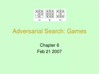
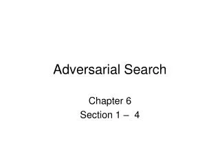
Adversarial Search. In this lecture, we introduce a new search scenario: game playing two players, zero-sum game, (win-lose, lose-win, draw) perfect accessibility to game information (unlike bridge) 4. Deterministic rule (no dice used, unlike Back-gammon).

E N D
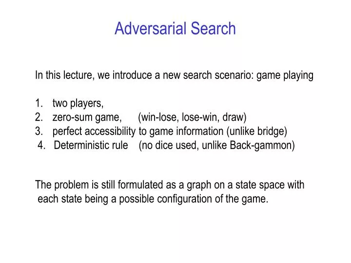
Adversarial Search • In this lecture, we introduce a new search scenario: game playing • two players, • zero-sum game, (win-lose, lose-win, draw) • perfect accessibility to game information (unlike bridge) • 4. Deterministic rule (no dice used, unlike Back-gammon) The problem is still formulated as a graph on a state space with each state being a possible configuration of the game.
The Search Tree MAX MIN MAX MIN We call the two players Min and Max respectively. Due to space/time complexity, an algorithm often can afford to search to a certain depth of the tree.
Game Tree Then for a leave s of the tree, we compute a static evaluation function e(s) based on the configuration s, for example piece advantage, control of positions and lines etc. We call it static because it is based on a single node not by looking ahead of some steps. Then for non-terminal nodes, We compute the backed-up values propagated from the leaves. For example, for a tic-tac-toe game, we can select e(s) = # of open lines of MAX --- # of open lines of MIN e(s) = 5 – 4 =1 S =
Alpha-Beta Search During the min-max search, we find that we may prune the search tree to some extent without changing the final search results. Now for each non-terminal nodes, we define an a and a b values A MIN nodes updates its b value as the minimum among all children who are evaluated. So the b value decreases monotonically as more children nodes are evaluated. Its a value is passed from its parent as a threshold. A MAX nodes updates its a value as the maximum among all children who are evaluated. So the a value increases monotonically as more children nodes are evaluated. Its b value is passed from its parent as a threshold.
Alpha-Beta Search We start the alpha-beta search with AB(root, a= - infinity , b= +infinity), Then do a depth-first search which updates (a, b) along the way, we terminate a node whenever the following cut-off condition is satisfied. b <= a A recursive function for the alpha-beta search with depth bound Dmax
Float: AB(s,a, b) • { if (depth(s) == Dmax) return (e(s)); // leaf node • for k =1 to b(s) do // b(s) is the out-number of s • {s’ := k-th child node of s • if (s is a MAX node) • { a := max(a, AB(s’, a, b)) // update a for max node • if ( b <= a) return (a); // b –cut • } • else • {b := min(b, AB(s’, a, b)) // update b for min node • if (b <= a) return (b); // a –cut • } • } // end for • if (s is a MAX node) return (a); // all children expanded • else return (b); • }