Download
1 / 15
150 likes | 283 Views
Course Outline. Overview of probability and statistics Microarray data analysis Protein function analysis based on the homology model Protein structure analysis Protein docking. Introduction to Microarray Data Analysis. Microarray Data Analysis.

E N D
Course Outline • Overview of probability and statistics • Microarray data analysis • Protein function analysis based on the homology model • Protein structure analysis • Protein docking
Microarray Data Analysis • In a microarray data set, each object is described by one row of gene expression values. • For example, in the Leukemia data set, there are 72 samples and 7129 genes. • 25 Acute Myeloid Leukemia(AML) samples. • 38 B-cell Acute Lymphoblastic Leukemia samples. • 9 T-cell Acute Lymphoblastic Leukemia samples.
Model of Microarray Data Sets Class 1 Class 2 Class 3
Data Classification • In a data classification problem, each object is described by a set of attribute values and each object belongs to one of the predefined classes. • The goal is to derive a set of rules that predicts which class a new object should belong to, based on a given set of training samples. Data classification is also called supervised learning.
Applications of Data Classification in Microarray Data Analysis • In microarray data analysis, data classification is employed to predict the class of a new sample based on the existing samples with known class. • In this regard, each object is described by one row of gene expression data in the microarray data table.
For example, in the Leukemia data set, there are 72 samples and 7129 genes. • 25 Acute Myeloid Leukemia(AML) samples. • 38 B-cell Acute Lymphoblastic Leukemia samples. • 9 T-cell Acute Lymphoblastic Leukemia samples.
The Vector Space Model • In the vector space model, each object is described by a number of numerical attributes/features. • For example, the outlook of a man is described by his height, weight, and age.
Each object therefore is associated with a coordinate in the vector space and the vector corresponding to the coordinate is called the feature vector of the object. • For example, the feature vector of the outlook of a man is <height, weight, age>. • It is typical that the objects are described by a large number of attributes/features.
Transformation of Categorical Attributes into Numerical Attributes • Represent the attribute values of the object in a binary table form as exemplified in the following:
Assign appropriate weight to each column. • Treat the weighted vector of each row as the feature vector of the corresponding object.
The Similarity/Dissimilarity Matrix Model • In this model, a matrix records the similarity/dissimilarity scores between every pair of objects.
Given the feature vector of each object, we can derive a dissimilarity matrix by treating the distance between a pair of objects as the dissimilarity score. We can then define the similarity score to be the reciprocal or some other function value of the dissimilarity score. • However, given a similarity/dissimilarity matrix, we may not be able to project all the objects in a vector space.
For example, assume that the matrix shown above records the distances between 6 objects. Then, we have distance(P1,P4) = 862 > distance(P1,P5) + distance(P4,P5) = 35 + 291
However, we may select P2, P5, P6 as representatives and use the distances to these representatives to describe an object. • For example, the feature vectors of P1 and P2 are <53, 35, 180> and <0, 816, 606>, respectively.