Download
1 / 36
370 likes | 572 Views
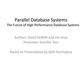
Parallel Database Systems Analyzing LOTS of Data Jim Gray Microsoft Research. Main Message. Technology trends give many processors and storage units inexpensively To analyze large quantities of data sequential (regular) access patterns are 100x faster

E N D
Parallel Database SystemsAnalyzing LOTS of DataJim GrayMicrosoft Research
Main Message • Technology trends give • many processors and storage units • inexpensively • To analyze large quantities of data • sequential (regular) access patterns are 100x faster • parallelism is 1000x faster (trades time for money) • Relational systems show many parallel algorithms.
1GB 128MB 1 chip memory size ( 2 MB to 32 MB) 8MB 1MB 128KB 8KB 1980 1990 2000 1970 bits: 1K 4K 16K 64K 256K 1M 4M 16M 64M 256M Moore’s Law • XXX doubles every 18 months 60% increase per year • Micro Processor speeds • chip density • Magnetic disk density • Communications bandwidthWAN bandwidth approaching LANs.
Magnetic Storage Cheaper than Paper • File Cabinet: cabinet (4 drawer) 250$ paper (24,000 sheets) 250$ space (2x3 @ 10$/ft2) 180$ total 700$3 ¢/sheet • Disk: disk (4 GB =) 500$ ASCII: 2 m pages(100x cheaper)0.025 ¢/sheet • Image: 200 k pages(10x cheaper).25 ¢/sheet • Store everything on disk
15 4 10 10 12 2 10 10 9 0 10 10 6 -2 10 10 3 -4 10 10 Today’s Storage Hierarchy : Speed & Capacity vs Cost Tradeoffs Price vs Speed Size vs Speed Cache Nearline Offline Tape Main Tape 1 Secondary Disc Online $/MB Online Size(B) Secondary Tape Tape Disc Main Offline Tape Nearline Tape Cache -9 -6 -3 0 3 -9 -6 -3 0 3 10 10 10 10 10 10 10 10 10 10 Access Time (seconds) Access Time (seconds)
ThesisMany Little will Win over Few Big 1 M$ 100 K$ 10 K$ Micro Nano Mini Mainframe 1.8" 2.5" 3.5" 5.25" 9" 14"
1k SPECint CPU 500 GB Disc 2 GB RAM Implications of Hardware Trends Large Disc Farms will be inexpensive (10k$/TB) Large RAM databases will be inexpensive (1K$/GB) Processors will be inexpensive So building block will be a processor with large RAM lots of Disc lots of network bandwidth CyberBrick™
Implication of Hardware Trends: Clusters CPU 50 GB Disc 5 GB RAM Future Servers are CLUSTERS of processors, discs Distributed Database techniques make clusters work
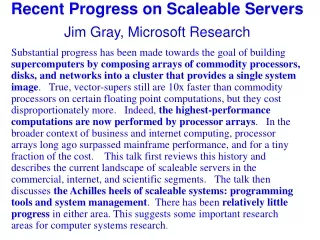
Summary • Tech trends => pipeline & partition parallelism • Lots of bytes & bandwidth per dollar • Lots of latency • Lots of MIPS per dollar • Lots of processors • Putting it together Scaleable Networks and Platforms • Build clusters of commodity processors & storage • Commodity interconnect is key (S of PMS) • Traditional interconnects give 100k$/slice. • Commodity Cluster Operating System is key • Fault isolation and tolerance is key • Automatic Parallel Programming is key
Parallelism: Performance is the Goal Goal is to get 'good' performance. • Law 1: parallel system should be • faster than serial system • Law 2: parallel system should give • near-linear scaleup or • near-linear speedup or • both.
Kinds of Parallel Execution Pipeline Any Any Sequential Sequential Program Program Sequential Sequential Any Any Sequential Sequential Sequential Sequential Partition outputs split N ways inputs merge M ways Program Program
The Perils of Parallelism Startup: Creating processes Opening files Optimization Interference: Device (cpu, disc, bus) logical (lock, hotspot, server, log,...) Skew: If tasks get very small, variance > service time
Why Parallel Access To Data? At 10 MB/s 1.2 days to scan 1,000 x parallel 1.5 minute SCAN. Bandwidth Parallelism: divide a big problem into many smaller ones to be solved in parallel.
Data Flow ProgrammingPrefetch & Postwrite Hide Latency Can't wait for the data to arrive(2,000 years!) Memory that gets the data in advance( 100MB/S) Solution: Pipeline from storage (tape, disc...) to cpu cache Pipeline results to destination Latency
Parallelism: Speedup & Scaleup Speedup: Same Job, More Hardware Less time 100GB 100GB Scaleup: Bigger Job, More Hardware Same time 1 TB 100GB Transaction Scaleup: more clients/servers Same response time 1 k clients 10 k clients 1 TB 100GB Server Server
Benchmark Buyer's Guide • Things to ask • When does it • stop scaling? • Throughput numbers, • Not ratios. • Standard benchmarks allow • Comparison to others • Comparison to sequential Ratios & non-standard benchmarks are red flags.
Why are Relational OperatorsSo Successful for Parallelism? • Relational data modeluniform operators • on uniform data stream • closed under composition • Each operator consumes 1 or 2 input streams • Each stream is a uniform collection of data • Sequential data in and out: Pure dataflow • partitioning some operators (e.g. aggregates, non-equi-join, sort,..) • requires innovation • AUTOMATIC PARALLELISM
Database Systems “Hide” Parallelism • Automate system management via tools • data placement • data organization (indexing) • periodic tasks (dump / recover / reorganize) • Automatic fault tolerance • duplex & failover • transactions • Automatic parallelism • among transactions (locking) • within a transaction (parallel execution)
Automatic Parallel OR DB Select image from landsat where date between 1970 and 1990 and overlaps(location, :Rockies) and snow_cover(image) >.7; Temporal Spatial Image • Assign one process per processor/disk: • find images with right data & location • analyze image, if 70% snow, return it Landsat Answer date loc image image 33N 120W . . . . . . . 34N 120W 1/2/72 . . . . . .. . . 4/8/95 date, location, & image tests
Automatic Data Partitioning Split a SQL table to subset of nodes & disks Partition within set: Range Hash Round Robin Good for equi-joins, range queries group-by Good for equi-joins Good to spread load Shared disk and memory less sensitive to partitioning, Shared nothing benefits from "good" partitioning
0...9 10..19 20..29 30..39 40.. A..C G...M D..F S..Z N...R Index Partitioning • Hash indices partition by hash • B-tree indices partition as a forest of trees. • One tree per range • Primary index clusters data
A..Z A..Z A..Z A..Z A..Z Base Table A..C G...M D..F S.. N...R Secondary Index Partitioning • In shared nothing, secondary indices are Problematic • Partition by base table key ranges • Insert: completely local (but what about unique?) • Lookup: examines ALL trees (see figure) • Unique index involves lookup on insert. • Partition by secondary key ranges • Insert: two nodes (base and index) • Lookup: two nodes (index -> base) • Uniqueness is easy • Teradata solution Base Table
N X M Data Streams M Consumers N producers River Data Rivers: Split + Merge Streams • Producers add records to the river, • Consumers consume records from the river • Purely sequential programming. • River does flow control and buffering • does partition and merge of data records • River = Split/Merge in Gamma = Exchange operator in Volcano.
Partitioned Execution Spreads computation and IO among processors Partitioned data gives NATURAL parallelism
N x M way Parallelism N inputs, M outputs, no bottlenecks. Partitioned Data Partitioned and Pipelined Data Flows
Picking Data Ranges • Disk Partitioning • For range partitioning, sample load on disks. • Cool hot disks by making range smaller • For hash partitioning, • Cool hot disks by mapping some buckets to others • River Partitioning • Use hashing and assume uniform • If range partitioning, sample data and use • histogram to level the bulk • Teradata, Tandem, Oracle use these tricks
Blocking Operators = Short Pipelines • An operator is blocking, • if it does not produce any output, • until it has consumed all its input • Examples: • Sort, • Aggregates, • Hash-Join (reads all of one operand) • Blocking operators kill pipeline parallelism • Make partition parallelism all the more important. Database Load Template has three blocked phases Sort Runs Table Insert Tape Scan Merge Runs SQL Table File SQL Table Process Sort Runs Index Insert Merge Runs Index 1 Sort Runs Index Insert Merge Runs Index 2 Merge Runs Sort Runs Index Insert Index 3
Simple Aggregates (sort or hash?) • Simple aggregates (count, min, max, ...) can use indices • More compact • Sometimes have aggregate info. • GROUP BY aggregates • scan in category order if possible (use indices) • Else • If categories fit in RAM use RAM category hash table • Else • make temp of <category, item> • sort by category, • do math in merge step.
Parallel Aggregates • For aggregate function, need a decomposition strategy: • count(S) = count(s(i)), ditto for sum() • avg(S) = ( sum(s(i))) / count(s(i)) • and so on... • For groups, • sub-aggregate groups close to the source • drop sub-aggregates into a hash river.
River is range or hash partitioned Merge runs Sub-sorts generate runs Range or Hash Partition River 6 log(10 ) 6 = => 2x slower Scan or other source 12 log(10 ) 12 Parallel Sort M inputs N outputs Disk and merge not needed if sort fits in memory Scales “linearly” because • Sort is benchmark from hell for shared nothing machines • net traffic = disk bandwidth, no data filtering at the source
Hash Join: Combining Two Tables Right Table • Hash smaller table into N buckets (hope N=1) • If N=1 read larger table, hash to smaller • Else, hash outer to disk then • bucket-by-bucket hash join. • Purely sequential data behavior • Always beats sort-merge and nested • unless data is clustered. • Good for equi, outer, exclusion join • Lots of papers, • products just appearing (what went wrong?) • Hash reduces skew Hash Buckets Left Table
Parallel Hash Join • ICL implemented hash join with bitmaps in CAFS machine (1976)! • Kitsuregawa pointed out the parallelism benefits of hash join in early 1980’s (it partitions beautifully) • We ignored them! (why?) • But now, Everybody's doing it. • (or promises to do it). • Hashing minimizes skew, requires little thinking for • redistribution • Hashing uses massive main memory
What Systems Work This Way • Shared Nothing • Teradata: 400 nodes • 80x12 nodes • Tandem: 110 nodes • IBM / SP2 / DB2: 128 nodes • Informix/SP2 100 nodes • ATT & Sybase 8x14 nodes • Shared Disk • Oracle 170 nodes • Rdb 24 nodes • Shared Memory • Informix 9 nodes • RedBrick ? nodes
Outline • Why Parallelism: • technology push • application pull • Parallel Database Techniques • partitioned data • partitioned and pipelined execution • parallel relational operators
Main Message • Technology trends give • many processors and storage units • inexpensively • To analyze large quantities of data • sequential (regular) access patterns are 100x faster • parallelism is 1000x faster (trades time for money) • Relational systems show many parallel algorithms.