Download

1 / 18
180 likes | 252 Views
Two Sample Tests. Nutan S. Mishra Department of Mathematics and Statistics University of South Alabama. Points to ponder. µ 1 =µ 2 can be rewritten as µ 1 -µ 2 =0 µ 1 < µ 2 can be rewritten as µ 1 -µ 2 < 0 µ 1 > µ 2 can be rewritten as µ 1 - µ 2 > 0 Equivalent values in.

E N D
Two Sample Tests Nutan S. Mishra Department of Mathematics and Statistics University of South Alabama
Points to ponder • µ1=µ2 can be rewritten as µ1-µ2 =0 • µ1< µ2 can be rewritten as µ1-µ2 < 0 • µ1 > µ2 can be rewritten as µ1 - µ2 > 0 • Equivalent values in
Description of the problem • There are two populations 1 and 2 • Parameters of 1 are (µ1,σ1) and that of 2 are (µ2,σ2) • We want to compare the average performances of these two populations. • That is we want to test if µ1=µ2 • In other words-- to test if µ1-µ2 =0
Description of the problem • Recall that at this point the true values of µ1 and µ2 are unknown. • But we are not interested in knowing the absolute values of µ1 and µ2 • We are interested in estimating and testing about the difference between the two namely µ1-µ2 • In order to conduct this test of hypothesis we collect two samples of size n1 and n2. • Samples collected may be dependent or independent.
Dependent samples Dependent samples : selection of one sample affects the selection of the other. Example: collecting data on length of sleep hours of insomnia patients before and after certain medication. First sample consists of values (3.2, 4.5, 4.5, 4.7) and the second samples consists of values (4.8, 5.3, 4.2, 4.7) Note that both samples are of same size n1 = n2
Independent samples Selection of one sample is independent of the other. Example: collecting data on emission of harmful gases from the vehicles in the state of California and in the state of Alabama Sample S1 consists of emission data on n1 vehicles from the state of California Sample S2 consists emission data on n2 vehicles from the state of Alabama. n1 may or may not be equal to n2 We may collect a sample of 100 vehicles from one state and a sample of 85 vehicles from the other.
Testing of hypothesis We will discuss them as different cases as follows
Testing hypothesis about difference of means There are two populations 1 and 2 • Parameters of 1 are (µ1,σ1) and that of 2 are (µ2,σ2) • Sample statistics are (n1, , s1) and (n2, , s2) • To test H0: µ1=µ2 equivalently H0: µ1-µ2 =0 • The point estimator for µ1-µ2 is • The test statistic would be • When σ12 and σ22are unknown we replace them by their point estimators namely s12 and s22 and the test statistic becomes
Exercise 10.11 X= hotel room rate per day in united states 1: all such room rates in 2000 (parameters (µ1,σ1) ) 2 : all such room rates in 2001 ( parameters (µ2,σ2)) To test H0: µ1=µ2 Vs H1: µ1 > µ2 equivalently we want To test H0: µ1 - µ2 =0Vs H1: µ1 - µ2 > 0 To test these hypotheses, two samples are collected from the respective populations with the following statistics: Sample S1 (from first population) = ( n1= 1000, = 85.69, s1 = 18.50) Sample S2(from second population= ( n2 = 1100, = 84.58 s2 = 18.00) The statistic would be It’s a right tailed hypothesis thus the p-value corresponding to z = 1.39 (from normal table ) is .0823 Since p-value > .01 ( which is given LOS) we decide not to reject H0 And conclude that at 1% LOS, the data supports the null hypothesis, that is room rates in 2000 and 2001 were not significantly different.
Two small independent samples There are two populations 1 and 2 • Parameters of 1 are (µ1,σ1) and that of 2 are (µ2,σ2) • Sample statistics are (n1, , s1) and (n2, , s2) • To test H0: µ1=µ2 equivalently H0: µ1-µ2 =0 • The point estimator for µ1-µ2 is For small n1 and (or) n2 , the test statistic is developed under following assumptions • Both populations are approximately normal • The population variances for both populations are unknown and EQUAL σ1 = σ2 ( say both of them equal to σ which is unknown) If these conditions are fulfilled then we can estimate the common unknown parameter σ by pooling the information (that is data coming from both samples) and call that estimate as pooled estimate of σ
Two small independent samples Now we define the test statistic under the two above conditions
Exercise 10.28(b) 1 : male customers at a supermarket 2: female customers at the same super market. XF= amount spent by a female customer. XM= amount spent by a male customer µM : average amount spent by all the male customers ( value is unknown) µF : average amount spent by all the female customers (value is unknown) σM: population standard deviation of male population spending ( value is unknown) σF: population standard deviation of female population spending ( value is unknown) Assumptions: 1. XM and XF have normal distribution . 2. σM = σF (both are unknown) let us say σM = σF =σ To test H0: µM =µF Vs H1: µM < µF in other words To test H0: µM -µF =0 Vs H1: µM-µF < 0
Exercise 10.28(b) (continued) Two samples are collected, one from each population. Information from samples: nM = 25 ( a sample of 25 males) = $80 average spending by 25 males sM = $17.50 sample standard deviation of spending of 25 males nF = 20 ( a sample of 20 females) = $96 average spending by 20 females sF = $14.40 sample standard deviation of spending of 20 females Now since both the samples are small, under the two assumptions above, the test statistic would be.
Exercise 10.28(b) (continued) Value of t-test statistic would be To compute sp Plugging in the value of Sp in the above formula we get the t-value as at 5% LOS the value of t at 43 d.f. is (from table) = 1.645 Since the alternative is left sided, our critical region lies in the left tail and the critical value is – 1.645. Comparing is the test statistic with the critical value, we see that test statistics falls in the rejection region
Exercise 10.28(b) (continued) Thus we make a decision to reject the H0 at 5% Level of significance Conclusion: We conclude that at 5% LOS, the sample data does not support the null hypothesis, this implies that the average spending by male customers is significantly lower than average spending by female customers.
Paired t-test Designed to compare the averages of two populations when two samples drawn are dependent ( or matched samples or paired samples). Here the population consists of same members (or objects or items) We collect two observations on each member of the population– before the treatment and after the treatment. Thus we generate two samples. X1: observation before the treatment X2: observation after the treatment d= difference in the measurement = x2-x1 d is a new random variable with µd = average of all the differences σd = standard deviation of all d-values in the population = mean of the d-values from the two samples each of size n sd = sample standard deviation of all d-values obtained from the two samples To test the hypothesis H0 : µd = 0 vs H1: µd < or > or ≠ 0 Under the assumption that population of all d-values is approximately normal, the test statistics is
Paired t-test (continued) The test statistics
Exercise 10.55(b) X1 : self confidence score before attending the course (scale 1-15) X2: self confidence score after attending the course (scale 1-15) d= x2-x1 = change in the confidence score after attending the course H0: µd = 0 vs H1: µd > 0 = 1.42857, sd = 1.988 test statistic Now since alternative hypothesis is right sided, the critical region lies on the right side of the t-curve. The critical value of t at 1% LOS is = 3.143 Comparing the critical value with test statistic, we observe that test statistic falls in non rejection region thus we make a decision not to reject null at 1% LOS since at 1% LOS sample data supports the null , we conclude that the course is not much effective as far as improvement in the confidence scores is concerned.