Download
1 / 58
580 likes | 758 Views
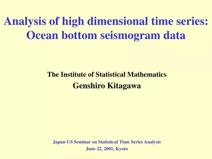
Analysis of high dimensional time series: Ocean bottom seismogram data. The Institute of Statistical Mathematics Genshiro Kitagawa Japan-US Seminar on Statistical Time Series Analysis June 22, 2001, Kyoto. T. Takanami, H. Shimamura (Hokkaido University) S. Watanabe

E N D
Analysis of high dimensional time series: Ocean bottom seismogram data The Institute of Statistical Mathematics Genshiro Kitagawa Japan-US Seminar on Statistical Time Series Analysis June 22, 2001, Kyoto
T. Takanami, H. Shimamura (Hokkaido University) S. Watanabe (Graduate Univ. for Advanced Study) (Schlumberger)
Example Exploring Underground Structure by OBS (Ocean Bottom Seismogram) data T. Takanami and H. Shimamura Hokkaido Univ., Inst. Seismologyand Volcanology
Exploring Underground Structure by OBS (Ocean Bottom Seismogram) Data Sea Surface OBS Bottom
4 Channel Time Series N=15360, 98239 series Experiment • Off Norway(Depth 1500-2000m) • 39 OBS, (Distance: 10-30km) • Air-gun Signal from a Ship (982 times: Interval 70sec., 200m) • Observation(dT=1/256sec., T =60sec., 4-Ch)
0 100 200 300 400 500 600 700 800 900 OBS-31 data K=982, N=15360
Time Adjustment • Cross-Correlation • Locally stationary AR model
Objectives Estimation of Underground Structure Detection of Reflection & Refraction Waves Estimation of parameters (hj, vj)
t-p Transformation x: Epicentral distrance t;Travel time p: Slowness t: Origin travel time Slant Stacking
Inverset-p Transformation Hilbert Transform Inverse of t-p
t-p filtering (OBS4) 0-150, 1-2000 150-320, 1-2000 320-400, 1-2000
t-p filtering (OBS4) 320-400, 1-200 0-150, 601-1000 0-150, 400-1200 150-320, 1-200
t-p filtering (OBS‐31) Original 160-200, 1-3000 0-160, 1-3000
Time-Varying AR model Model for the coefficients State Space Representation Power Spectrum
Time-Varying Spectrum Ch-700 Ch-720 Ch-740 Ch-760
Time-Varying Spectrum Ch-700 Ch-720 Ch-740 Ch-760
Time series at hypocenter (D=0) Wave(011) Wave(00011) Wave(0) Wave(000) Wave(00000)
Model for Decomposition Self-Organizing Model
State Vector Change of Variance Self-organizing SSM Self-organizing State Space Model
Nonlinear Non-Gaussian State Space Model State Time Series Non-Gaussian System Noise Non-Gaussian Observation Noise
Monte Carlo Filter System Noise Predictive Distribution Importance (Bayes) Factor Filter Distribution(by Resampling)
Reflection Wave Direct Wave Tau 1 Tau 2 Decomposition of Ch-701 Observed
Reflection Wave Direct Wave Decomposition of Ch-721 Observed
Modeling Spatial-Temporal Structure • Correlation structure between adjacent series • Time-space model
Modeling Space-Time Structure Multivariate Time Series Time Series Structure Relation Between Adjacent Series Time Series Model Spatial Model Spatio-Temporal Model
Model of Propagation Path Parallel Structure Width Velocity
Examples of Wave Path Wave(0) Wave(000) Wave(01) Wave(011) Wave(0121) Wave(000121) Wave(01221) Wave(012321) Wave(00012321)
Time Series at Wave(0) Wave(000) Wave(00000)
Velocity of Water Wavev0 a=-0.060
Path Models and Arrival Times Arrival Time(Sec.) ーD/6 Distance(km)
Path models and arrival times(OBS4) Arrival Time (sec.) Distance (km)
Spatial Filter k:Time-lag
Spatial Model(Ignoring time series structure) Series j-1Series j : Time-lag=k
Kalman-like Filter Initial Prediction Prediction Filter Filter
Path Models and the Differences of the Arrival Times Between Adjacent Channels Epicentral Distance
8 7 6 5 4 3 2 1 0 Arrival Time -10 -8 -6 -4 -2 0 2 4 6 8 10 D: Distance Local Time Lag
Estimation of Time Lag Log-likelihood Local log-likelihood
OBS4 SHIFT=23
OBS4 SHIFT=13 SHIFT=8 SHIFT=3