Download
1 / 49
530 likes | 926 Views
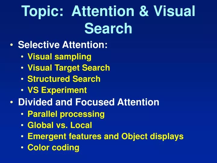
Topic: Attention & Visual Search. Selective Attention: Visual sampling Visual Target Search Structured Search VS Experiment Divided and Focused Attention Parallel processing Global vs. Local Emergent features and Object displays Color coding. Attention Types. Selective Attention

E N D
Topic: Attention & Visual Search • Selective Attention: • Visualsampling • Visual Target Search • Structured Search • VS Experiment • Divided and Focused Attention • Parallel processing • Global vs. Local • Emergent features and Object displays • Color coding
Attention Types • Selective Attention - Visual sampling behavior : A searchlight metaphor • Focused Attention - To concentrate on one source of information in the environment • Divided Attention - Aspect of attention that enables us to do multiple tasks or attend to multiple stimuli at the same time
Visual SamplingProcess • Foveal Vision and Peripheral Vision • About 2 degree of visual angle (Foveal vision) : To keep objects in foveal vision • The other is peripheral visions • Pursuit and saccade eye movement • Pursuit: Following a target moving at a constant speed • Saccade Movement: A series of discrete, jerky movements that jump from one point to the other • Useful field of view (Visual lobe) • Diameter around the central location from which information is extracted) • Dwell time • How long the eye remains at that location
Target Search • Free search is sequence of eye movements. • Eye moves in saccades, about 3/s in free search, more in display processing, more for confirmation of target • Information intake inversely proportional to eye movement speed (graph) • Therefore information processing at fixations with little during eye movements • Effectively, series of still photos
What can we see in one fixation? • We can deduce that for any target size, there is an area around the line of sight (fixation point) within which we can see the target. • This is called the Useful Field of View (UFOV) or Visual Lobe (VL) • Inside VL, target visible, outside not • VL typically elliptical around line of sight
Given size UFOV or VL
UFOV or VL Eye Search Field
Some Search Findings • People tend to search center more than periphery • People use prior probabilities to structure search, looking first where p(target) is greatest. • Visual Lobe size varies with target conspicuity, or target / background contrast • Visual Lobes usually about 1o to 10o
Visual search models • Two issues: • Search process over multiple fixations • Information processing within one fixation • Two limiting processes in free search: random and systematic • Random means no memory for previous fixations, therefore can re-visit • Systematic means perfect memory and no revisits • Sampling with or without replacement
Random Search Model • If p(detect) on any one fixation is p • p(detect on fixation 1) = p • p(detect on fixation 2) = p(1-p) • p(detect on fixation 3) = p(1-p)(1-p) • p(detect on fixation i) = p(1-p)i-1 • thus diminishing returns over successive fixations • We really need the Cumulative probability of detection up to fixation n
…continued • P(detect up to and including fixation n) = P(n) = p(1-p)i-1 for I = 1 to n • This is the same to P(n) = p(1-p)n • We can expand this as a series, and approximate terms in the series to give • P(n) = 1 - exp (-np) • If fixations take a constant time, then we can express P(n) as P(t) • P(n) = 1 - exp (-t) where = 1/mean time
Some Facts • This graph tells us the performance in terms we want, i.e. how many targets will be detected in a given time • This is a negative exponential distribution • Only one parameter, thus all functions the same shape, just differ in X-axis scale • Neg. Exp. Distribution has mean = standard deviation = 1/
Systematic search • Assume as before, p(detect) in any fixation = p • If complete coverage takes M fixations, then for fixations between 0 and M, Cumulative p(detect) is linear of slope p • P(n) = pn/M • After one complete scan, operator probably tries another scan, and so on until detection • If M = 5 and p = 0.181 (same as random)
Systematic Search P(t) = np/M Random Search P(t) = 1 - exp (- 0.2 t)
Notes on search • If same p(detect) = p, both systematic and random start from same origin with same slope. • Systematic curve always better than random, higher P(t) for any t > 0 • How do people really search? • Systematic and random give limits. Real performance between these limits • Arani, Karwan, Drury (HF, 26, 1984, p631) developed a variable memory model
Uses of Search Models • Give performance / time curves to show cost of achieving given reliability • Example from steel inspection data: fits well to random search model • Can see reliability consequences of limited time • Can use models plus costs to find optimum search time, or Stopping Policy
Simple Stopping Time • Let Value of search success = V and cost of search failure = C • Let cost of searching for time t = kt • E(Value) = V(1- exp (-t) ) - C exp (-t) - kt • Max (E(Value) = dE/dt • dE/dt = V exp (-t) + C exp (-t) - kt • At t=topt, dE/dt = 0 • Solving gives: topt = Log ( (V+C)/k) • Optimum time longer for large , large V+C, small k. has double effect
List Search • If search field is a list, then get special effects • Examples are checking lottery numbers, menus on computer screens • Usually strict serial scan: time to detect target = k * target position • Neisser search task • Plot time vs position, slope = k • Gives speed of processing each item
Menu Search • If items listed randomly, user must read down using Neisser search technique • If embedded menus, 3 - 10 items per menu is optimum for search speed • Can locate by frequency of use to minimize overall search time • If not randomly listed, then search can be much faster, e.g. telephone book listing, items positions consistent e.g. Windows • Depends on learned ordering, e.g. A,B,C,..
Visual Search Exp. • In free search field • Geometric Mean search times (GMST) • 산술평균은 visual search performance의 특성을 제대로 반영하지 못함 • 지수분포의 평균값 구하기와 유사 • Visual search performance는 여러 가지 변수에 따라 달라짐 • Field의 복잡성 • Target과 배경의 상관관계 • 인간의 Search 방법 등 등
Divided Attention and Parallel Processing • So far we have considered a purely serial process with each area searched in turn until search terminates with success or at Stopping Time • Parallel Processing이 되면, 한번의 Fixation에서 많은 양의 정보 그리고 다양한 정보를 처리할 수 있다. • 즉 Divided attention (분산주의) 을 하고 있다. - 한 단어속의 모든 문자는 병렬로 처리됨
Parallel Processing • Occurs by direct perception of a feature of the target which “pops out” of the display • Perceptual organization is closely related: how we use our world model to simplify • Pre-attentive is another word. Implies that processing occurs without the need for attentional resources • Examples: • Array of instruments organized by type or shape: grouping • Instruments where pointers line up if all is OK, so that deviant pointer “pops out”
Pointer Line-up, Pop out
Parallel vs Serial Process • 일반적으로 두 단계의 시각정보 처리과정을 거친다. • Parallel 과 serial processing • 예) 배경과 object의 구별 : Parallel Processing • But under some circumstances we find parallel processing. • Trivial case: if target very salient, then VL always includes target and thus one fixation always finds target
Spatial Proximity • Spatial proximity can help divided attention • But not always • Sometimes cause errors • Pilots are shown critical instrument readings on the glass windscreen to ensure simultaneous processing without visual scanning (Fig. 3.9) • Proximity of irrelevant signs can inhibit response to signal • Response conflict results if perceptual channels are close together and have incompatible implications for action e.g. Stroop task
Say the color of text • XXXXX • XXXXX • WHITE • BLUE • RED • YELLOW • GREEN • RED • BLUE
Stroop Effect • Comes from conflict between highly-learned responses • Would not cause a problem in an unknown foreign language! • If word and color agree, we have facilitated response from redundancy gain
Object display and proximity compatibility • Object displays are displays that have integral dimensions • The proximity of compatibility principle states that the benefit of presenting dimensions (information source) in an integrated format will depend on the extent to which the information from these sources must be integrated
Applications • Summary: Scale goes from: • Focused attention where one channel is attended and others must be suppressed • Divided attention where multiple channels must be attended to together • Where we need focused attention avoid clutter and competing dimensions • Where we need divided attention, integrate the dimensions so that new perception (Gestalt) emerges
Examples • Use of integral dimensions: • Aircraft attitude indicator gives pitch, yaw and roll relative to straight ahead and horizon • Polyhedron display for many parameters in complex process control tasks • Height X Weight = Area for some applications
항공기의 비행자세 디스플레이와 안전변수 디스플레이
Rate Area = total ventilation Volume
Color Coding • Single color is always preattentive, and gives parallel search • Useful redundancy, e.g. traffic signals • But don’t overdo it! Canbevery distracting if irrelevant. PowerPoint may have hundreds of colors but you do NOT have to use them all!
Graph Display • Most useful display depends upon the task • Do you want accurate reading of specific data point, or comparison of two data points or overall picture? • Best display different for each • Task Proximity is the issue • Example: Single readings followed by integration over several data points: PowerPoint Default gradually improved
Remove Unnecessary 3-D Effect for easier reading of single points
Lines better for perceiving relationships between data points
Legend Removed and labels placed by lines, lines bolder North West East
Y-axis grid lines removed to emphasize pattern, I.e. trends North West East
Changes • Second graph good for reading values • Later graphs better for perceiving patterns • Keep labeling consistent • Highlight differences • Use labeled scales “Sales” vs. “1999 quarter” • Use proper scale values and ranges: scales in units of 1, 2 or 5 x 10n. Start at true zero or indicate non-zero start by scale break