Download
1 / 42
430 likes | 444 Views
Parallel Graph Algorithms. Graph Algorithms. Minimum Spanning Tree (Prim’s Algorithm) Single-Source Shortest Path (Dijkstra’s Algorithm) All-Pairs Shortest Paths (Dijkstra’s and Floyd’s Algorithm). Adjacency Matrix. An adjacency matrix represent the edges of a graph. Adjacency Matrix.

E N D
Graph Algorithms • Minimum Spanning Tree (Prim’s Algorithm) • Single-Source Shortest Path (Dijkstra’s Algorithm) • All-Pairs Shortest Paths (Dijkstra’s and Floyd’s Algorithm)
Adjacency Matrix • An adjacency matrix represent the edges of a graph
Adjacency Matrix • Example 0 1 2 1 2 4 3 3 4 2
Prim’s Algorithm for Minimum Spanning Tree V – set of vertices VT – set of vertices in the MST E – set of edges A – adjacency matrix r – root node d – minimum distance from MST to any vertex Prim_MST(V, E, A, r) { VT = {r}; d[r] = 0; for all v in (V – VT) d[v] = Ar,v; while (VT != V) { Find a vertex u such that d[u] = min(d[v] for all v in (V – VT)); VT = VT + {u}; for all v in (V – VT) { d[v] = min(d[v], Au,v); } } } Complexity = O(n2)
Root is node b(Prim’s) a 3 Initialize 1 f 3 b 5 c 5 1 2 1 d e 4 Since d[3] = 1, add the edge b to d and consider node d next
Next consider node d(Prim’s) a 3 Take Minimums except for b and d 1 f 3 b 5 c 5 1 2 1 d e 4 Since d[0] = 1, add the edge b to a and consider node a next
Next consider node a (Prim’s) a 3 1 f 3 b 5 c 5 1 2 1 d e 4 Since d[2] = 2, add the edge d to c and consider node c next
Next consider node c(Prim’s) a 3 1 f 3 b 5 c 5 1 2 1 d e 4 Since d[4] = 1, add the edge c to e and consider node e next
Next consider node e(Prim’s) a 3 1 f 3 b 5 c 5 1 2 1 d e 4 Since d[5] = 3, add the edge a to f and consider node f next
Next consider node f(Prim’s) a 3 1 f 3 b 5 c 5 1 2 1 d e 4 VT= V so stop
Parallelizing Prim’s Algorithm • We can’t just simply execute the while loop in parallel because the d[] array changes with each selection of a vertex • We have to update values in d[] from all processors after each iteration • Suppose we have n vertices in the graph and p processors
Parallelizing Prim’s Algorithm • Partition and adjacency matrix and the distance array (d) across processors d[ ] n A 0 1 2 p-1
Parallelizing Prim’s Algorithm • Each processor computes the next vertex from among its vertices • A reduction is done on the distance array (d) to find the minimum • The result is broadcast out to all the processors
Prim’s Algorithm (Parallel) Prim_MST(V, E, A, r) { ... // Initialize d as before #pragma paraguin begin_parallel while (VT != V) { Find a vertex u such that d[u] = min(d[v] for all v in (V – VT)); VT = VT + {u}; #pragma paraguin forall for v in V if (v VT) d[v] = min(d[v], Au,v); #pragma paraguin reduce min d #pragma paraguin bcast d } #pragma paraguin end_parallel }
Prim’s Algorithm (Parallel) • Complexity of Parallel algorithm: • Each reduction and broadcast takes log p time, but we have to do up to n of them. Communication Computation
Dijkstra’s Algorithm for Single-Source Shortest Path • Given a source node, what is the shortest distance to each other node • The minimum spanning tree gives is this information
Dijkstra’s Algorithm V – set of vertices VT – set of vertices in the MST E – set of edges A – adjacency matrix r – root node d – minimum distance from root to any vertex Dijkstra_SP(V, E, A, r) { VT = {r}; d[r] = 0; for v in (V – VT) d[v] = Ar,v; while (VT != V) { Find a vertex v such that d[u] = min(d[v] for all v in (V – VT)); VT = VT + {u}; for v in (V – VT) d[v] = min(d[v], d[u] + Au,v); } } Complexity = O(n2) This is the only thing different
Source Node is node b(Dijkstra’s) a 3 Initialize 1 f 3 b 5 c 5 1 2 1 d e 4 Since d[3] = 1, consider node d next
Next consider node d(Dijkstra’s) a 3 1 f 3 b 5 c 5 1 2 1 d e 4 Since l[0] = 1, consider node a next
Next consider node a(Dijkstra’s) a 3 1 f 3 b 5 c 5 1 2 1 d e 4 Since l[2] = 3, consider node c next
Next consider node c(Dijkstra’s) a 3 1 f 3 b 5 c 5 1 2 1 d e 4 Since l[4] = 4, consider node e next
Next consider node e(Dijkstra’s) a 3 1 f 3 b 5 c 5 1 2 1 d e 4 Since d[5] = 4, add the edge a to f and consider node f next
Next consider node f(Dijkstra’s) a 3 1 f 3 b 5 c 5 1 2 1 d e 4 VT= V so stop
Parallelizing Dijkstra’s Algorithm • Since Dijkstra’s Algorithm and Prim’s Algorithm are essentially the same, we can parallelize them the same way: • Complexity of Parallel algorithm: • If we have n processors, this becomes: Communication Computation
All Pairs Shortest Path • Dijkstra’s Algorithm gives us the shortest path from a particular node to all the others • For All Paris Shortest Path, we want to find the shortest path between all pairs of vertices • We can apply Dijkstra’s Algorithm to every pair of vertices • Complexity = O(n3)
All Pairs using Dijkstra’s Algorithm V – set of vertices VT – set of vertices in the MST E – set of edges A – adjacency matrix r – root node d – minimum distance from root to any vertex Dijkstra_APSP(V, E, A) { for r in V { VT = {r}; d[r] = 0; for all v in (V – VT) d[v] = Ar,v; while (VT != V) { Find a vertex u such that d[u] = min(d[v] for all v in (V – VT)); VT = VT + {u}; for v in (V – VT) d[v] = min(d[v], d[u] + Au,v); } } } Complexity = O(n3)
All Pairs Shortest Path • We can parallelize the outermost loop • Each processors assumes a different node vi and computes the shortest path to all nodes • No communication if needed • Complexity is O(n3/p) • If we have n processors, complexity is O(n2) • If we have n2 processors, we can use n processors for each vertex. Complexity becomes O(nlogn)
Floyd’s Algorithm for All Pairs Shortest Path • Floyd’s Algorithm works off of this observation: • Consider a subset of V: • Let be the weight of the shortest path from vi to vj that includes one of the vertices in • If vk is not in the shortest path from vi to vj, then • Otherwise, the shortest path is
Floyd’s Algorithm for All Pairs Shortest Path • This leads to the following recurrence: • We can implement this using iteration and not recursion
All Pairs using Floyd’s Algorithm Floyd_APSP(V, E, A) { d0i,j = Ai,j for all i,j for k = 1 to n for i = 1 to n for j = 1 to n d(k)i,j = min(d(k-1)i,j , d(k-1)i,k + d(k-1)k,j ) • We don’t need n copies of the d matrix. We only need one. • In fact, we can do it with only one matrix V – set of vertices E – set of edges A – adjacency matrix Complexity = O(n3)
Partitioning of the d matrix • We divide the d matrix into p blocks of size n/√p • Each processor is responsible for n2/√p elements of the d matrix … … … …
Partitioning of the d matrix • However, we have to send data between processors k column j column k row i row
Communication Pattern … … … …
Analysis of Floyd’s Algorithm • Each processor has to send its block to all processors on the same row and column. • If we use a broadcast, then the time to communication is • The synchronization step requires • The time to compute the values for each processors is
Analysis of Floyd’s Algorithm • So the complexity for each step is: • And finally, the complexity for n steps (of the k loop) is: Communication Computation
A faster version of Floyd’s Algorithm • We can do a pipeline of values moving through the matrix. • The reason is because once processor pi, j computes the value of it can then send it to the processors pi, j-1 , pi, j+1 , pi+1, j , and pi-1, j
Consider the movement of the value computed by processor 4 Time t t+1 t+2 t+3 t+4 1 2 3 4 5 6 7 8 Processors
Analysis of Floyd’s Algorithm with pipelining • The net complexity of the algorithm using pipelining is: Communication Computation