Download
1 / 28
280 likes | 600 Views
Autocorrelation. The randomness of the sample implies that the error terms for different observations will be uncorrelated.

E N D
The randomness of the sample implies that the error terms for different observations will be uncorrelated. When we have time-series data, where the observations follow a natural ordering through time, there is always a possibility that successive errors will be correlated with each other. In any one period, the current error term contains not only the effects of current shocksbut also the carryover from previous shocks. This carryover will be related to, or correlated with, the effects of the earlier shocks. When circumstances such as these lead to error terms that are correlated, we say that autocorrelation exists. The possibility of autocorrelation should always be entertained when we are dealing with time-series data. The Nature of Autocorrelation
For efficiency (accurate estimation / prediction) all systematic information needs to be incorporated into the regression model. Autocorrelation is a systematic pattern in the errors that can be either attracting (positive) or repelling (negative) autocorrelation.
crosses line not enough (attracting) et . . . . . . . Postive Auto. . . . . . . . 0 . . . . . . . . t crosses line randomly et . . . . . . . . . . . . No Auto. . . . . . . . . . 0 . . . . . . t . crosses line too much (repelling) . . et . . . . . . . Negative Auto. . . 0 . . . . . t . .
cov(et, es) = t=s cov(et, es) = t=s Regression Model yt = 1 + 2xt + et E(et) = 0 zero mean: homoskedasticity: var(et) = 2 nonautocorrelation: autocorrelation:
Order of Autocorrelation yt = 1 + 2xt + et 1st Order: et = et1+ t et = 1et1 + 2et2+ t 2nd Order: 3rd Order: et = 1et1 + 2et2 + 3et3 + t We will assume First Order Autocorrelation: et = et1 + t AR(1):
cov(t, s) = t=s First Order Autocorrelation yt = 1 + 2xt + et et = et1 + t where 1 < < 1 var(t) = 2 E(t) = 0 These assumptions about t imply the following about et: E(et) = 0 cov(et, etk) = e2 kfor k>0 2 var(et) = e2 = corr(et, etk) = kfor k>0 12
If we have an equation whose errors exhibit autocorrelation, but we ignore it, or are simply unaware of it, what does it have on the properties of least squares estimates? 1. The least squares estimator is still linear andunbiased but it is not efficient. 2. The formulas normally used to compute the least squares standard errors are no longer correct and confidence intervals and hypothesis tests using them will be wrong. Autocorrelation creates someProblems for Least Squares:
yt = 1 + 2xt + eAutocorrelation:E(et) = 0, var(et) = 2, cov(et, es) = ,t s • (Linear) Where (Unbiased)
var(b2) = xt x yt = 1 + 2xt + et cov(et, es) = ,t s Autocorrelation: Incorrect formula for least squares variance: e2 Correct formula for least squares variance:
Generalized Least Squares AR(1) : et = et1 + t substitute in for et yt = 1 + 2xt + et yt = 1 + 2xt + et1 + t Now we need to get rid of et1 (continued)
yt = 1 + 2xt + et1+ t yt = 1 + 2xt + et lag the errors once et = yt12xt et1 = yt112xt1 yt = 1 + 2xt + yt112xt1+ t (continued)
* yt = 1 xt1*+ 2 xt2* + t , * yt = yt yt1 xt2 = (xtxt1) * x1t* = (1) yt = 1 + 2xt + yt112xt1+ t yt = 1 + 2xt + yt112xt1+ t yt yt1 = 1(1) + 2(xtxt1)+ t t =2, 3, …, T.
1. One observation is used up in creating the transformed (lagged) variables leaving only (T1) observations for estimating the model (Cochrane-Orcutt method drops the first observation). 2. The value of is not known. We must find some way to estimate it. * yt = yt yt1 xt2 = xt xt1 * * yt = 1 xt1*+ 2 xt2* + t , x1t* = (1) Problems estimating this model with least squares:
(Option) Recovering the 1st Observation Dropping the 1st observation and applying least squares is not the best linear unbiased estimation method. Efficiency is lost because the variance of the error associated with the 1st observation is not equal to that of the other errors. This is a special case of the heteroskedasticity problem except that here all errors are assumed to have equal variance except the 1st error.
Recovering the 1st Observation The 1st observation should fit the original model as: y1 = 1 + 2x1 + e1 with error variance: var(e1) = e2 = 2 /(1-2). We could include this as the 1st observation for our estimation procedure but we must first transform it so that it has the same error variance as the other observations. Note:The other observations all have error variance2.
y1 = 1 + 2x1 + e1 with error variance: var(e1) = e2 = 2/ (1-2). The other observations all have error variance 2. Given any constant c : var(ce1) = c2 var(e1). If c = 1-2 , then var( 1-2 e1) = (1-2) var(e1). = (1-2) e2 = (1-2) 2/(1-2) = 2 The transformation 1= 1-2e1 has variance 2 .
y1 = 1 + 2x1 + e1 Multiply through by 1-2 to get: 1-2y1 = 1-21 + 1-22x1 + 1-2 e1 The transformed error 1= 1-2e1 has variance 2 . This transformed first observation may now be added to the other (T-1) observations to obtain the fully restored set of T observations.
* yt = 1 xt1*+ 2 xt2* + t , We can summarize these results by saying that, providing is known, we can find the Best Linear Unbiased Estimator for 1 and 2 by applying least squares to the transformed mode t =1, 2, 3, …, T. where the transformed variables are defined by for the first observation, and for the remaining t = 2, 3, …, T observations.
^ et = ytb1b2xt Estimating Unknown Value If we had values for the et , we could estimate: et = et1 + t First, use least squares to estimate the model: yt = 1 + 2xt + et The residuals from this estimation are:
^ et = yt - b1 - b2xt ^ ^ et = et1 + t ^ ^ T et et-1 ^ t = 2 = ^ T et-1 2 t = 2 Next, estimate the following by least squares: The least squares solution is:
Durbin-Watson Test The Durbin-Watson test is by far the most important one for detecting AR(1) errors. It is assumed that the vt are independent random errors with distribution N(0, v2). The assumption of normally distributed random errors is needed to derive the probability distribution of the test statistic used in the Durbin-Watson test.
^ ^ T et et-1 2 d= t = 2 ^ T et 2 t = 1 The Durbin-Watson Test statistic, d, is: For a null hypothesis of no autocorrelation, we can use H0: = 0. For an alternative hypothesis we could use H1: > 0 or H1: < 0 or H1: 0.
^ The test statistic, d, is approximately related to as: 0 d 2(1) 4 ^ When = 0 , the Durbin-Watson statistic is d 2. ^ ^ When = 1 , the Durbin-Watson statistic is d 0. When = 1, the Durbin-Watson statistic is d 4. Testing for Autocorrelation ^ Tables for critical values for d are not always readily available so it is easier to use the p-value that most computer programs provide for d. Reject H0 if p-value < , the significance level.
Test for the first-order autocorrelation Reject H0 Inclusive Do not reject H0 H1: > 0 d < dL dL < d < dUd > dU H1: < 0 d > 4 dL 4 dU < d < 4 dLd < 4 dU d > 4 dL 4 dU < d < 4 dL H1: 0 or or dU < d < 4 dU d < dL dL < d < dU Note: The lower and upper bounds (dL and dU) depend on sample size n and the number of explanatory variables k (not include intercept).
A. Test for Positive Autocorrelation > 0 No evidence of positiveautocorrelation Inclusive 0 dU 2 dL 4 B. Test for Negative Autocorrelation No evidence of negative autocorrelation Inclusive < 0 2 4 dU 4 dL 4 0 C. Two-Sided Test for Autocorrelation No evidence of autocorrelation > 0 Inclusive < 0 Inclusive 2 4 dL dU 4 dU 4 0 dL
^ ^ ^ ~ ^ yT+1 = 1 + 2xT+1 + eT ^ ^ where 1and 2 are generalized least squares estimates and eT is given by: ~ Prediction with AR(1) Errors When errors are autocorrelated, the previous period error may help us predict next period error. The best predictor, yT+1 , for next period is: ^ ^ ~ eT = yT12xT
^ ^ ^ ~ ^ yT+h = 1 + 2xT+h + h eT ~ ^ ^ Assuming | | < 1, the influence of h eT diminishes the further we go into the future (the larger h becomes). For h periods ahead, the best predictor is: