Download
1 / 47
480 likes | 639 Views
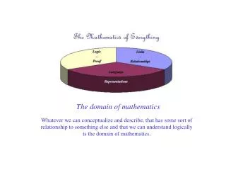
The domain of mathematics. Whatever we can conceptualize and describe, that has some sort of relationship to something else and that we can understand logically is the domain of mathematics. Algorithms for Functions (recursive and iterative). Computer representation of numbers and text.

E N D
The domain of mathematics Whatever we can conceptualize and describe, that has some sort of relationship to something else and that we can understand logically is the domain of mathematics.
Algorithms for Functions (recursive and iterative) Computer representation of numbers and text Logic, Sets, Boolean algebra, Predicates and Proofs Relations, equivalence, ordering, graphs and trees ReviewDiscrete Mathematics for Computing
Algorithms for Functions (recursive and iterative) Computer representation of numbers and text Logic, Sets, Boolean algebra, Predicates and Proofs Relations equivalence, ordering graphs and trees Algorithms and Functions
Algorithms • An algorithm is a procedure to be followed, a sequence of steps to be executed by some agent, in order to achieve a certain function. • For example: First compute sb2- 4 a cThen test to see if s > 0 or s < 0 is true. If s is positive compute z (-b + s)/(2a) , (-b-s)/(2a) if not . . . • Certain data will need to be available, represented by (a,b,c) -- the input. • Certain data will be made available, represented by z--the output. • Intermediate variables such as s will not overwrite workspace variables (nor will a,b,c or z) if algorithm is declared as a function.
Function syntax • The syntax line:[0] y = fred (x,z) NB. or y = fred x, z • tells you that • the name of the function is fred, • the inputs are given in two variables called x and z which are unassigned variables for the purposes of the algorithm, • whatever the variable y holds at the end of the algorithm, that is the output. • The above is a pre-fix notation. Other notations are infix, e.g. x fred zpostfix, e.g. x z fred
[0] y= Pivot reduce Matrix[0.1]NB.Pivot is a location in Matrix[1] r first(Pivot) [2] c last(Pivot) [3] p Pivot entry_in Matrix[4] R r row_of Matrix[5] R R divided_by p . . . [n] NB. Output is a matrix y with ... This is a function with an infix syntax. Functions almost always call other functions. Supplied functions are the primitives of a language. [0] y = modulus x [0.1] NB.Input x is a vector[0.2] NB.Output y is mod of x [1] s square_each x[2] S sum s[3] y sqrt S This function has a pre-fix syntax. Some languages require parentheses, e.g.modulus(x), sqrt(S) etc. Defining a function
Recursive Functions • Some computing environments allow recursive functions, that is functions that call themselves at some stage of their execution.Successive calls must eventually lead to an exit condition (delivering a result).Consequently there must be a branching control structure that determines when this situation applies.
Fibonacci (recursive) function • [0] s = fibacci(a,b,n) • [0.1]NB. s is the list of n Fibonacci numbers starting with [a,b] • [1] If n = 2 NB. add escape line for n < 2 if desired • [1.1] sa, b • else • [1.2] sfibacci(a,b, n-1) • [1.3] ss, last(s) + last(curtail(s))
Lists • Iterative procedures and recursive functions often lead to the generation of numeric lists -- i.e. functions of the whole numbers. • Discrete mathematics is about functions of countable sets (or whole numbers). • List manipulating functions are central to discrete mathematics.
Recursive definition of lists • Lists are often defined recursively using index notation, for example:pn+1 = Gpn {first order linear iteration}pn+1 = Gpn(1- pn){first order non-linear} pn+2 = Gpn+1+ Hpn {second order linear} • Linear recurrence relations can be solved by assuming solutions of the form Acn
Control Structures • Branching controls (e.g. in recursive functions) • If {test(…)} do … else … • Iterative procedures and • While {test(…)} do … • Repeat … until {test(…)} • For c = a to b do …(Do-Loops) • test is a propositional function which for particular variable values returns 0 or 1.
[0] y R growth P[0.1] NB. R is a two element vector giving the growth rate of population with initial count of P and the number of years through which it will be traced. [1] g first (R) [2] n last(R)[3] y P [4] For i = 1 to n do [4.1] yy,(1+g/100)*last(y)[5]NB. Output is a list (vector) y [0] y Joh N[0.1] NB. N a natural number[1] If N = 1 do [1.1] y 1else [1.2] If N =2*floor(N/2) do [1.2.1] y(2*Joh N/2) - 1else [1.2.2] y(2*Joh floor N/2)+1 [2] NB. y is the output This function has a pre-fix syntax. Iterative and recursive functions Some languages require parentheses, e.g. Joh(x), floor(S) etc.
[0] Joh(26)[2.2.1] y(2*Joh 26/2) - 1 [0] Joh(13) [2.2.2] y(2*Joh floor 13/2)+1 [0] Joh(6) [2.2.2] y(2*Joh 6/2)-1 [0] Joh(3) [2.2.2] y(2*Joh floor 3/2)+1 [0] Joh(1) [2.1] y 1 [2.2.2] y2*1 + 1 [0] 3 {Joh(3)} [2.2.2] y2*3 - 1 [0] 5 {Joh(6)} [2.2.2] y2*5 + 1 [0] 11 {Joh(13)} [2.2.2] y2*11 - 1 [0] 21 {Joh(26)} Tracing a function's execution
Algorithms for Functions (recursive and iterative) Computer representation of numbers and text Logic, Sets, Boolean algebra, Predicates and Proofs Relations equivalence, ordering graphs and trees Computer representation of data
The symbol set • Each symbol of a symbol set (the alphabet, numerals, special characters) is represented by a binary code. • The ASCII code is a fixed length (8-bit) code. • Huffman codes are variable length codes with the shorter lengths for the most common symbols in a particular setting.
8 bit ASCII • 00110101 = (0011)(0101) = 3516 = 48+5 = 5310 represents the numeral '5' (as distinct from the number 5). • 01000101 = (0100)(0101) = 4516 = 64+5 = 6910 represents the letter 'E'. • 0100010100110101 represents 'E5' (4535 in hex)
0 1 A 1 0 O 1 0 R 1 0 S T Huffman Codes • Huffman codes encode characters by using variable length codes designed for a particular application, the length of each code depending on the frequency of the character's use. • e.g. 01010111 using • the binary treeshown represents RAT
Binary Representation • The electrical abacus. • Place value:26+24+23+22 = 921011100 = 1.26 +0.25 +1.24 +1.23+1.22 +0.21+0.20= 2(1.25 +0.24 +1.23 +1.22+1.21 + 0)+ 0= 2(2(1.24 +0.23 +1.22 +1.21+1)+ 0)+ 0 = 2(2(2(1.23 +0.22 +1.21 +1) +1)+ 0)+ 0 = 2(2(2(2(1.22 +0.21 +1)+1) +1)+ 0)+ 0= 2(2(2(2(2(1.21 +0)+1)+1) +1)+ 0)+ 0= 2(2(2(2(2(2(1)+0)+1)+1) +1)+ 0)+ 0
Fractional Numbers • 0.101101 = 1/2 + 1/23+1/24+1/26 = 45/64 • 0.011 = 1/22 + 1/23 = (2+1)/8 = 3/8 = 0.375 • 0.375 = (0 + 0.75)/ 2 = (0 + (1 + 0.5)/ 2)/ 2 = (0 + (1 + (1 + 0)/ 2)/ 2)/ 2 = 0.011 • 0.0246 0.0492 0.0984 0.1968 0.3936 0.7872 1.5744 1.1488 0.2976 0.5952 1.1904 0.3808 = 0.00000110010…= 1/64+1/128+1/1024 + …= (16+8+1)/1024 +… = 25/1024 + … = 0.02441406…
Octal / Binary conversions • 8=23 so binary numbers broken into groups of three will give the octal equivalents: 101 011 001 010 100 (binary) is 5 3 1 2 4 (octal)and, conversely octal numbers can be easily converted to binary: 6 5 7 . 3 2 (octal) is 110 101 111. 011 010 (binary)
Hexadecimal /Binary conversions • 16=24 so binary numbers broken into groups of four will give the hex equivalents: 1010 0110 1101 0101 (binary) is A 6 D 5 (hex)and, conversely hex numbers can be easily converted to binary: B 5 E . 3 F (hex) is 1011 0101 1110 . 0011 1111 (binary)
Octal and Hexadecimal system • The major uses of octal and hex are as shorter versions for binary numbers. • Converting to decimal: B5E.3F is 11*162+5*16+14+3/16+15/162= 11*256+80+14+(48+15)/256= 2905. 24609375 • Decimal to octal or hex is the same as for binary except now divide (and multiply) by 8 and 16 respectively instead of by 2.
Integers in a computer • Integer arithmetic in a computer is a modular arithmetic to a base like 216i.e. Z65536 . • Numbers up to 32767 have binary representations beginning with a 0 e.g. 0111111111111111 while numbers larger than this i.e. numbers n with a leading one, e.g. 1000000000000000 represent the negative numbers n-216 = -m. • Since n=216-m = 1+ 1111111111111111-m it is the 2's complement of m.
Computer Representations of Integers • Positive numbers:0 0 0 0 0 0 0 0 0 0 0 1 1 1 1 0sign bit binary representation of number • Negative numbers:1 1 1 1 1 1 1 1 1 1 1 0 0 0 1 0sign bit 2's complement (2k-m) of modulus • Subtraction by adding 2's complement.
Computer Representations of Reals • Normalized binary exponential form e.g.:0.1001011110011011 x 212 • Exponent bias 2m-1-1 where m is the number of bits for the characteristic. (e.g. m = 8) • Characteristic is 12 + 27-1 = 10001011 • Sign bit; characteristic, mantissa filled with trailing zeros if necessary: • 0 10000111 1001011110011011 0000000
Computer Arithmetic • Integer arithmetic is exact, but floating point arithmetic is subject to representation and round-off errors. • Notice that real number arithmetic is done in exponential (or polar) form: • (a 2u) + (b 2v) = [ a 2(u-v)+b ] 2v (a 2u) x (b 2v) = a b 2u+v • Multiplying by 2m is a shift in the binary point.
Comparison tolerance • Since there is a largest and a smallest number that any computer can hold, we may have overflow if we exceed the largest or underflow if we try to get closer to 0 than the smallest. • Comparison tests such as a > b ; a = b or a- b = 0are usually effected with a a pre-set tolerance. Note that the last two may not be equivalent if the comparison tolerance is a proportional one.
Algorithms for Functions (recursive and iterative) Computer representation of numbers and text Logic, Sets, Boolean algebra, Predicates and Proofs Relations equivalence, ordering graphs and trees Logic, Sets and Boolean Algebra Predicates and Proofs
The Laws of Logic • These are the laws of a Boolean Algebra: • [commutativity] p+q = q+p ; p q = q p • [associativity] p+(q+r) = (p+q)+r ; p (q r) = (p q) r • [distributivity] p+q r = (p+q)(p+r) ; p (q+r) = p q + p r • [identity elements] 0, 1 such that: • p + 0 = p ; p 1 = p ; p+p' = 1 ; p p' = 0 • where ' represents the negation operator ; + represents and multiplication (elided) represents , 0 is a contradiction, 1 a tautology. • DeMorgan (p+q)' = p'q' ; (pq)' = p'+q' and all other laws, such as 1' = 0; 0' = 1; p+1=1; p 0 = 0 ; p+p= p ; etc., may all be deduced from the above.
Predicates and Quantifiers • A predicate is completed and becomes a proposition if • all variables are given specific values • each variable is quantified by specifying that either there exists some value () for which the predicate is true or that the predicate is asserted to be true for all values () of the variable. • [ gP(g)] g [ P(g)] ; [ gP(g)] g [ P (g)] [ g ( P(g))] gP(g); [ g ( P(g))] gP (g)
Strategies for Proof • Given a set of assumptions (axioms or accepted truths), showing that a proposition is logically equivalent to some subset of the axioms constitutes a proof. • Showing that the negation of a proposition is equivalent to a contradiction of the axioms is also a proof. • Showing that there is one value of the variable for which the predicate is not true is a proof that the predicate is not true for all values of the variable.
If P(0) is true P(n) P(n+1) then P(N) is true for all N Proof by Induction • If the truth of proposition, P(n), implies the truth of P(n+1) • andP(n0) is true • thenP(n) is true for all n n0.
Sets and Cartesian Products • the null set, Ø , • the universal set, • complement of a set, • disjoint sets, • partitions of a set, • cardinality of a set, • the union, intersection and equality of sets, • the power set and • the cartesian product of sets.
Laws of Operation with Sets • These are the laws of a Boolean Algebra: • [commutativity] A+B = B+A ; A B = B A • [associativity] A+(B+C) = (A+B)+C ; A(BC) = (AB)C • [distributivity] A+B C = (A+B)(A+C) ; A (B+C) = A B+A C • [identity elements] 0, 1 such that: • A + 0 = A ; A 1 = A ; A+A' = 1 ; A A' = 0 • where ' represents the complementation operator C ; + represents and multiplication (elided) represents , 0 is the empty set, and 1 the universal set . • DeMorgan (A+B)' = A'B' ; (AB)' = A'+B' and all other laws, such as 1' = 0; 0' = 1; A+1=1; A 0 = 0 ; A+A= A ; etc., may all be deduced form the above.
Boolean Algebra • These are the laws of a Boolean Algebra: • [commutativity] x+y = y+x ; x y = y x • [associativity] x+(y+z) = (x+y)+z ; x (y z) = (x y) z • [distributivity] x+y z = (x+y)(x+z) ; x (y+z) = x y + x z • [identity elements] 0, 1 such that: • x + 0 = x ; x 1 = x ; x+x' = 1 ; x x' = 0 • where ' represents the unary operator and + and multiplication (elided) represents binary operators. • DeMorgan (x+y)' = x'y' ; (xy)' = x'+y' and all other laws, such as 1' = 0; 0' = 1; x+1=1; x 0 = 0 ; x+x= x ; etc., may all be deduced form the above.
zw z'w z'w' zw'xy 1 0 0 0 x'y 0 1 0 0x'y' 1 1 0 1xy' 1 0 0 1 Karnaugh Maps and Circuits • The Karnaugh map is a technique for identifying factors such as (x+x')y =1y=y in Boolean expressions. • It relies on functions being written in disjunctivenormalform, the sum of minterms that can be read from the function table. • Logic circuits are constructed using not, and and or gates.
Algorithms for Functions (recursive and iterative) Computer representation of numbers and text Logic, Sets, Boolean algebra, Predicates and Proofs Relations, equivalence, ordering, graphs and trees Relations and Graphsfunctional: one depends on the otherequivalence: in some sense the sameordering: can be compared in some way.
Relations and Functions • A Boolean algebra is a set, B, with a unary (BB) and two binary (BBB) functions (operations), that are both commutative, associative and distributive over each other and with elements 0 and 1 for which x + 0 = x ; x 1 = x and x + x' = 1 ; x x' = 0. • A binary relationship on B is a subset of BB. The relationship holds if some test (propositional function) returns true. • y = 2x+3 defines a binary relationship on R (true for points on a line). The test is an equality. f(x)=2x +3 defines unary function; (x2+y2) defines a binary function on R. Output: a number.
Equivalence Relations • A relation ~ is an equivalence relation on set S • if and only if it is • symmetric a ~ b b ~ a • transitive (a ~ b) (b ~ c) a ~ c • reflexive a ~ a • forall a, b, c in S. • Irreflexive means that there are no elements in S for which a ~ a .
Ordering Relations • A partial ordering, @, on a set S, • has the properties of • reflexivity a @ a • transitivity a @ b b @ c a @ c • anti-symmetry a @ b b @ a a = b • forall a, b, c in S. • {Note the use of infix notation for these relations.}
Graphs and Circuits • Graphs consist of vertices and edges. Graphs can be represented by adjacency matrices. • The sum of the degrees of the vertices of a graph is twice the number of edges in the graph. • In any graph the number of vertices with odd degree is even. (The 'Handshaking Lemma') • If all the vertices of G are of even degree, then the graph is Eulerian. If exactly two vertices of G have odd degree then the graph is semi-Eulerian. If G has more than two vertices of odd degree, the G is neither Eulerian nor semi-Eulerian (cf Hamiltonian paths).
Trees and Optimization • A tree is a connected graph with NO cycles. Adding an edge between two vertices of a tree will produce a cycle, removing an edge will result in a disconnected graph. • A tree with n vertices has n -1 edges and any graph with n vertices and n -1 edges is a tree. • A spanning tree is a connected sub-graph that contains all the vertices. Optimization problems with weighted graphs require minimal spanning trees.[Prim's and Kruskals algorithms; Dijkstra's algortihm for distance between vertices.]
Rooted Trees / Expression Trees • Decision trees are oftenbinary trees with left and rightchildren. • In-order traversal: ((a/b) + c) - (de) • Pre-order traversal:- + / abc de • Post-order traversal:a b / c + d e -