Download
1 / 10
100 likes | 231 Views
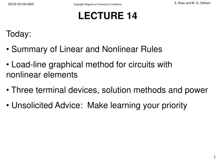
LECTURE 14. Today: Summary of Linear and Nonlinear Rules Load-line graphical method for circuits with nonlinear elements Three terminal devices, solution methods and power Unsolicited Advice: Make learning your priority. Reduce or eliminate: Over-focusing on policy and grades

E N D
S. Ross and W. G. Oldham LECTURE 14 • Today: • Summary of Linear and Nonlinear Rules • Load-line graphical method for circuits with nonlinear elements • Three terminal devices, solution methods and power • Unsolicited Advice: Make learning your priority
S. Ross and W. G. Oldham Reduce or eliminate: • Over-focusing on policy and grades • Better off devoting energy towards understanding • Perfectionism • Don’t expect perfection of yourself or your instructors • Competition • Cooperation, helping others benefits you too Big don’ts for success at school and at work Art, Michelle and Rob(Be Like Michelle)
S. Ross and W. G. Oldham Circuit Laws and Tricks • Linear Circuits: • KCL, KVL • Nodal Analysis • Thévenin and Norton equivalents • Nonlinear Circuits: • KCL, KVL • Nodal Analysis • Special Graphical Technique for Circuits containing linear and nonlinear elements (Load-line Method): • Combine all linear parts into a simple Thévenin equivalent Circuit attached to the nonlinear element. • Plot the I-V Characteristics of NLE and Thévenin circuit on same axes, recognizing the intersection as the solution.
S. Ross and W. G. Oldham 200K +- 2V ID D D Non-linear element NLE 1M + - 250K VDS 9mA +- S S Example of Load-Line Method We have a circuit containing a two-terminal non-linear element “NLE”, and some linear components. First replace the entire linear part of the circuit by its Thevenin equivalent. Then define I and V at the NLE terminals (typically associated signs) 1V
S. Ross and W. G. Oldham ID D N L E 200K 200K +- +- 2V 2V S ID ID (mA) D 10 NLE + - The solution ! VDS S VDS (V) 1 2 Example of Load-Line method (con’t) Given the graphical properties of two terminal non-linear circuit (i.e. the graph of a two terminal device) And have this connected to a linear (Thévenin) circuit Whose I-V can also be graphed on the same axes (“load line”) Application of KCL, KVL gives circuit solution
S. Ross and W. G. Oldham ID D 200K +- 2V S ID Application of KCL, KVL gives circuit solution (mA) 10 The solution ! VDS (V) 1 2 Load-Line method The method is graphical, and therefore approximate But if we use equations instead of graphs, it could be accurate It can also be use to find solutions to circuits with three terminal nonlinear devices (like transistors)
S. Ross and W. G. Oldham ID 3-Terminal Device D G S Three-Terminal Devices With three terminals we have four independent variables (two voltages and two currents) We can set one variable at each terminal and the I-V behavior of the device will determine the value of the two unknowns. For example apply a VGS and VDS, then measure IG and ID. Similarly we could apply a fixed VGS and IG and plot the two-terminal characteristic ID versus VDS.
S. Ross and W. G. Oldham ID 3-Terminal Device D G VGS = 3 +- VGS = 2 VGS S ID (mA) 10 VGS = 1 VDS (V) 1 2 Three-Terminal Parametric Graphs Concept of 3-Terminal Parametric Graphs: We set a voltage (or current) at one set of terminals (here we will apply a fixed VGS, IG=0) and conceptually draw a box around the device with only two terminals emerging so we can again plot the two-terminal characteristic (here ID versus VDS). But we can do this for a variety of values of VGS with the result that we get a family of curves.
S. Ross and W. G. Oldham G ID D S 200K +- V +- 2V ID ID VGS = 3 (mA) (mA) 10 VGS = 2 10 The solution ! VGS = 1 VDS VDS (V) 1 2 (V) 1 2 Graphical Solutions for 3-Terminal Devices We can only find a solution for one input (VGS) at at time: First select VGS (e.g. 2V) and draw ID vs VDS for the 3-Terminal device. Now draw ID vs VDS for the 2V - 200KW Thevenin source. The only point on the I vs V plane which obeys KCL and KVL is ID = 5mA at VDS = 1V.
S. Ross and W. G. Oldham ID D G Three-Terminal Devices – Power Flow IG 3-Terminal Device S With three terminals we have two independent measures of power (e.g. one at GS and one at DS). We can set any two variables and the I-V behavior of the device will determine the value of the other two. Defining all currents as inward, the power dissipated is simply the algebraic sum of VGS IG and VDS ID, i. e., P (in) = VGS IG + VDS ID . See the textbook, p. 117 for more generality.