Download
1 / 29
290 likes | 524 Views
Overview of Trend Analysis Selecting Indicators Assessing Uncertainties Adjusting for Meteorology Adjustment Techniques Important Meteorological Variables Example Met-adjustments Discerning Trends Graphical Methods Examples. Spatial Trends in PM Examples

E N D
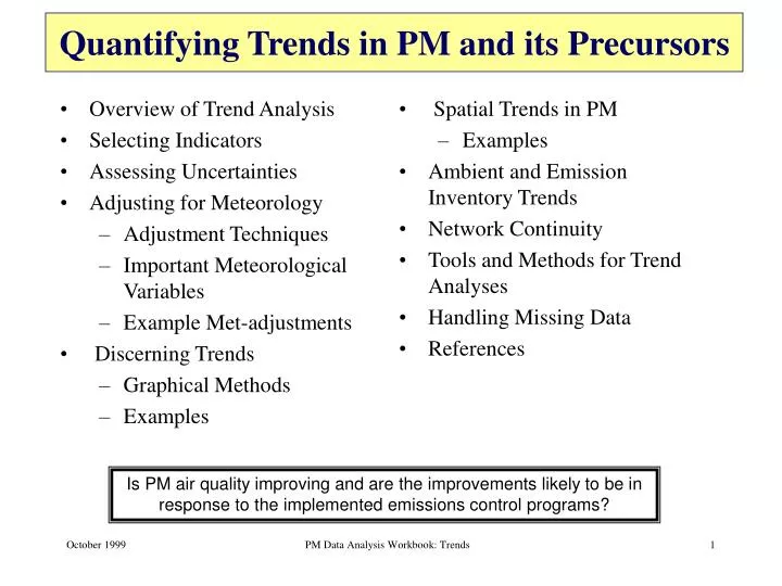
Overview of Trend Analysis Selecting Indicators Assessing Uncertainties Adjusting for Meteorology Adjustment Techniques Important Meteorological Variables Example Met-adjustments Discerning Trends Graphical Methods Examples Spatial Trends in PM Examples Ambient and Emission Inventory Trends Network Continuity Tools and Methods for Trend Analyses Handling Missing Data References Quantifying Trends in PM and its Precursors Is PM air quality improving and are the improvements likely to be in response to the implemented emissions control programs? PM Data Analysis Workbook: Trends
Overview of Trend Analysis (1 of 2) • Rationale for assessing trends in PM. One of the major objectives for routine PM2.5 speciation data is for the analysis of trends. • Indicator selection is important. Trends in extreme values in a data set may differ significantly from trends observed in a statistic that describes the bulk of the data. • Understanding the data uncertainties is necessary. Uncertainties could obscure our ability to discern air quality trends. • Changes in meteorology can obscure trends. Meteorology, which can significantly affect air quality, can vary among years. • Discerning trends can be tricky. PM Data Analysis Workbook: Trends
Overview of Trend Analysis (2 of 2) Rationale for assessing trends in PM. One of the major programmatic objectives for the routine PM2.5 chemical speciation is providing data for the analysis of air quality trends and to track progress of control programs. The ability to detect trends in ambient concentrations that are associated with planned air quality control efforts must be incorporated in State Implementation Plan assessments. For example, if specific control strategies have been implemented in an area to reduce fugitive emissions from construction activities, do the ambient data indicate lower concentrations of PM species associated with crustal material since the implementation of the control? Indicator selection is important. Air quality data typically do not fit a normal distribution. The data tend to be more skewed and exhibit a few high concentration events. Thus, trends in extreme values in a data set may differ significantly from trends observed in a statistic that describes the bulk of the data. Data can be statistically adjusted to assess trends in peak days and on more typical days. For example, one can plot the annual maximum PM concentrations to assess how annual peak days are changing over time or one can plot the median PM concentrations to assess how the 50th percentile of the days are changing. In addition, in order to assess a trend in air quality, sufficient data are required over a sufficient time period. Understanding the data uncertainties is necessary. Uncertainties impact the ability to clearly discern air quality trends. For example, measurement accuracy, precision, bias, and interferences need to be understood to properly interpret the data. Also uncertainties arising from compiling large amounts of measurements into a single performance indicator can be important. Changes in meteorology can obscure trends in air quality. We know that the meteorology among years can vary significantly (e.g., El Niño) and meteorology can have a significant affect on air quality. Therefore, when we assess trends in air quality, we need to be able to adjust the data to account for meteorological conditions that were very different from average conditions. By properly accounting for the portion of the variability in the data attributable to changes in meteorology, we can compare air quality among years with widely different meteorological conditions. This is important because we do not have control over how meteorology changes. Discerning trends can be tricky. The analyst needs to understand methods for quantifying trends and determining their statistical significance. The analyst also needs to be able to communicate the results in a meaningful and understandable way. US EPA, 1998 PM Data Analysis Workbook: Trends
Selecting Indicators (assuming 24-hr data) • Statistical indicators include: arithmetic mean, geometric mean, median, maximum, minimum, 2nd & 3rd maximums, selected percentiles. • Time periods over which to apply the statistics include: quarterly, seasonally, episode (i.e., days above some threshold) vs. non-episode, annually. • PM measurements upon which to apply the statistics include: mass, species groups (e.g., total metals), individual species (e.g., Pb), ratios of species. Concentrations and weight percent of total mass can be used. • Consensus among trends in indicators gives the analyst more confidence in the results. US EPA, 1998 PM Data Analysis Workbook: Trends
Assessing Uncertainties in Trend Analyses (1 of 2) • Uncertainties impact one’s ability to clearly discern air quality trends in an analysis. • Uncertainties that affect trends in air quality are: • Atmospheric variability associated with short-term fluctuations in meteorological conditions and source emissions. • Meteorological variability associated with synoptic seasonal cycles. • Measurement uncertainty associated with instrument accuracy and precision. • Analysis uncertainty associated with trend indicator interpretation • Methods exist to account for or adjust for variations in meteorology. PM Data Analysis Workbook: Trends
Assessing Uncertainties in Trend Analyses (2 of 2) Uncertainties impact one’s ability to clearly discern air quality trends in an analysis. Uncertainties place confidence limits on the parameters that are being analyzed and are needed to determine whether or not significant conclusions can be drawn from trends within the variability or uncertainty of the measurement. Some uncertainties that affect trends in air quality are: 1. Atmospheric variability associated with short-term fluctuations in meteorological conditions and source emissions. 2. Meteorological variability associated with synoptic seasonal cycles. 3. Measurement uncertainty associated with instrument accuracy and precision. 4. Analysis uncertainty associated with trend indicator interpretation. The first two uncertainties are the result of real atmospheric events and can impact long-term trending by introducing real variability into the measurements. Short-term atmospheric variability can be the result of meteorological or emission events that are uncommon (anomalous events) and result in measurements that are inconsistent from one day to the next. Meteorological variability is considered a result of changes in seasonal cycles. This type of uncertainty normally occurs on a longer time scale and is a result of changes in the measurements due to seasonal changes in meteorology. Both of these variabilities are the result of real atmospheric events and cause real uncertainties in the measurements. (This is contrary to the uncertainties that are a result of measurement and analysis techniques; these uncertainties are the result of a statistical uncertainty or artifact.) Many researchers have dedicated their time to developing methods to account for or adjust for these variations. For example, Larsen uses native variability and expected peak day concentrations to account for the effects of uncommon short-term atmospheric meteorological or emission fluctuations (e.g., California Air Resources Board, 1993). Cox and Chu adjust ozone and PM measurements to account for seasonal differences from year-to-year (e.g., Cox and Chu, 1993). Rao and Zurbenko adjust ozone measurements to account for differences from year-to-year in both atmospheric fluctuations and seasonal meteorology (e.g., Rao and Zurbenko, 1994). Many of the techniques were developed for application to ozone trends; however, these same techniques are beginning to be applied to PM trends. Wittig et al., 1999 PM Data Analysis Workbook: Trends
Adjusting for Meteorology Exploratory Investigation of PM2.5 Dependence on Meteorology on Washington DC IMPROVE Data • Adjustment techniques involve some processing of the PM measurements to remove the influence of particular events or conditions from the data prior to any trends analysis. • Adjustment techniques are compared in the following tables so that an analyst can decide which methods are the most reasonable to consider depending upon the data available. • The figure here illustrates some of the meteorological parameters that have an affect on PM2.5 concentrations. One of the next steps is whether or not these parameters show a significant interannual impact. Morning Mixing Height Avg. Daytime RH Approx. Fractional Change in PM2.5 Avg. Daytime Temp. Avg. Daytime Pressure Approx. Fractional Change in PM2.5 Cox et al., 1999 PM Data Analysis Workbook: Trends
Adjustment Techniques (1 of 3) PM Data Analysis Workbook: Trends Wittig et al., 1998
Adjustment Techniques (2 of 3) Wittig et al., 1998 PM Data Analysis Workbook: Trends
Adjustment Techniques (3 of 3) Wittig et al., 1998 PM Data Analysis Workbook: Trends
Important Meteorological Variables • Possible meteorological variables important to PM trend analysis include: daily average specific humidity, average morning (0600-0900) wind speed, average afternoon (1300-1600) wind speed, morning mixing height, average 1000-1600 relative humidity, daily average temperature, daily average barometric pressure, wind direction, transport/recirculation measures. • To assess possible important meteorological variables, the following analyses are helpful: examine a matrix of scatter plots of fine mass and all possible independent variables available, perform Classification and Regression Tree (CART) analysis, perform cluster or factor analysis; perform other multivariate analyses. • The correlation between some variables can be improved by offsetting ambient data and meteorological parameters by a lag time. Cox et al., 1998 PM Data Analysis Workbook: Trends
Example Meteorology-adjusted Trends Exploratory Investigation of PM2.5 Dependence on Meteorology on Washington DC IMPROVE Data 826 daily observations • In this example, a general linear model was developed in which each of the independent variables was modeled using a natural cubic spline with three degrees of freedom. Meteorological parameters were stepwise deleted from the full model. • The trend components with (twice standard errors) are shown here with and without meteorology included in the model. Important variables (averages) included: daily specific humidity, morning and afternoon wind speeds, morning mixing height, daytime relative humidity, and daytime surface temperature and pressure. • The meteorologically adjusted trends appear to be smoother and flatter than the non-adjusted trends. • The impact of interannual variations in meteorological conditions do not appear to be large enough to alter any conclusions about long-term PM trends at this site. Approx. Fractional Change in PM2.5 Approx. Fractional Change in PM2.5 Cox et al., 1999 PM Data Analysis Workbook: Trends
Discerning Trends • Linear Model: Use simple linear regression on annual summary statistics or to logged statistics (if lognormal); perform analysis of variance. • Nonparametric Methods: To test for and estimate a trend without making distributional assumptions (e.g., Spearman's rho test of trend, Kendall's tau test of trend). • Time Series Models: Statistical modeling of ozone concentrations taking into account their serial dependence (e.g., auto-regressive integrated moving average - ARIMA). • Extreme Value Theory: To estimate distributions of annual maximum hourly concentrations, estimate distributions of the number of days exceeding the standard (e.g., Chi-square test, Poisson process approximation). Stoeckenius et al., 1994 PM Data Analysis Workbook: Trends
Graphical Methods for Discerning Trends • Box plots (high and low values, median values, outliers) • Plots of mean or median values with confidence intervals • Line graph of selected indicator • Interpolated or contoured maps of PM indicators • Combination of map with temporal information PM Data Analysis Workbook: Trends
Using Box Plots to Investigate Trends • Box plots are useful for displaying trends in data. • Box plots illustrate the trends in the high values, the low values, and the means. • In this graph, the variability is about the same from year to year - the boxes for each year are about the same height. • Also note a gradual, steady downward trend over the years 1988-1997, for the high values, the low values, and the central values. • For PM, we’re interested in both the high, episodic values, and the annual means because PM has both chronic, long-term health effects and episodic, short-term health effects. US EPA, 1998 PM Data Analysis Workbook: Trends
Using Confidence Intervals to Investigate Trends Sample illustration of the use of confidence intervals to determine statistically significant changes. Confidence intervals are shown for 4 years of data. Since the plotted confidence intervals overlap for years 1 and 2 but not for years 1 and 3, years 1 and 2 are not significantly different, but years 1 and 3 are significantly different. US EPA, 1994 PM Data Analysis Workbook: Trends
Using Simple Line Graphs to Investigate Trends(1 of 2) Simple line graphs can be used to assess trends in selected indicators. In this graph, a map was combined with plots of the second maximum 8-hr CO concentration per year for each region. A similar plot could be prepared for PM2.5 concentrations. US EPA, 1998 PM Data Analysis Workbook: Trends
Using Simple Line Graphs to Investigate Trends(1 of 2) Long-term Ambient Pb Trend, 1977-1997 • It is sometimes useful to break a long-term trend into shorter time intervals because of significant changes in emissions. • For example, leaded gasoline was phased out starting in the late 1970s. Dramatic reductions were observed in ambient Pb concentrations up to the 1980s. Since the late 1980s, Pb concentrations are near detection. • Similar dramatic reductions in ambient benzene concentrations have been observed because of the introduction of reformulated fuels (e.g., Main et al., 1998). US EPA, 1998 PM Data Analysis Workbook: Trends
Spatial Trends in PM Average PM2.5 ConcentrationsJuly, August, September 1994-1996 • A comparison of PM indicators among sites can be performed using simple graphics and tables, sophisticated contoured maps, or techniques in between. This map shows significant differences in annual PM2.5 concentrations across the US. • It is important to use consistent data records (e.g., same site operating over all years of the trend period) when assessing spatial and temporal trends. • Spatial and temporal trend assessments can be combined. This is a work in progress. The map is currently the best available but is expected to change as estimation methods improve and additional data is incorporated. Falk, 1999 PM Data Analysis Workbook: Trends
IMPROVE Network PM2.5 Trends 1988-1997 • The map shows the annual trends in overall PM2.5 concentration for 1988-1997, at 34 monitoring sites in the continental U.S. which have been recording PM2.5 concentrations for over six years. • The site labels are the annual trends of PM2.5 concentrations at each site. The data were deseasonalized to "take out" the seasonal cycle of PM2.5. Frechtel et al., 1999 PM Data Analysis Workbook: Trends
Ambient and Emission Inventory Trends • It is important to compare ambient trends with trends in the emission inventory. Do the ambient trends corroborate changes in emissions? • The example here compares chemical mass balance model results for 1988 and 1993 (Southeast Michigan Ozone Study - SEMOS) in Wayne County Michigan. Vehicle exhaust concentrations (top) are nearly unchanged while gasoline vapor concentrations have declined. • Results are consistent with a significant reduction in gasoline Reid Vapor Pressure (RVP - a measure of volatility) between 1988 and 1993. Scheff et al., 1996 PM Data Analysis Workbook: Trends
Network Continuity Discussion and example to be added PM Data Analysis Workbook: Trends
Tools and Methods for Trend Analysis (1 of 2) Available mapping software includes: • Surfer (http://www.goldensoftware.com/) • MapInfo (http://www.mapinfo.com/) • ArcInfo (http://www.esri.com/) • SAS (http://www.sas.com/) • AIRS graphics • Other similar statistical and GIS-based software. PM Data Analysis Workbook: Trends
Tools and Methods for Trend Analysis (1 of 2) Available methods for trend analysis include (and example reference): • De-seasonalizing annual trends: Frechtel et al., 1999http://capita.wustl.edu/PMFine/Workgroup/Status&Trends/Reports/Completed/LongTermIMPROVE/LongTermIMPROVE.html • Assessing seasonal trends: Eldred, 1994 • Spatial estimation method: Capita, 1999http://capita.wustl.edu/SAPID/Summaries/SpatialEstimation/sld002.htm • Meteorological adjustment using filtering: Rao and Zurbenko, 1994 • Meteorological adjustment using probability distribution: Cox and Chu, 1998; Cox et al., 1999 http://capita.wustl.edu/OTAG/reports/otagwind/OTAGWIN4.html • Classification and regression tree analysis: Stoeckenius, 1990 PM Data Analysis Workbook: Trends
Handling Missing Data • In the assessment of long-term trends for the EPA trends report, analysts handle missing annual data in the following manner: • Missing the last year: set the missing year equal to the second-to-last year • Missing the first year: set the missing year equal to the second year. • Missing any other year: interpolate between the available two years. • Data handling conventions for missing data and for determining whether a site is in compliance with the NAAQS are discussed in detail in US EPA, 1999. PM Data Analysis Workbook: Trends
References Bloomfield P., Royle J.A., Steinberg L.J., and Yang Q. (1996) Accounting for meteorological effects in measuring urban ozone levels and trends. Atmos. Environ. 30, 3067-3077. Butler A . J ., Mulholland J . A ., Russell SA . G ., Tolbert P . E ., Wilkinson J . G . (1998) Temporal and Spatial Distributions of Ozone in Atlanta: Regulatory and Epidemiologic Implications. Journal of the Air & Waste Management Association. 48, 418 - 426. California Air Resources Board (1993) Guidance for using air quality-related indicators in reporting progress in attaining the State Ambient Air Quality Standards. Report prepared for the California Air Resources Board, Sacramento, CA., September. California Air Resources Board (1995) Air quality indicators for 1981 to 1993 to report progress in attaining the State ambient air quality standards for ozone, carbon monoxide, and nitrogen dioxide. Report prepared by the California Environmental Protection Agency Air Resources Baord, Air Quality Analysis Section, Technical Support Division, Sacramento, CA, September. California Air Resources Board (1997) California ambient air quality data: 1980-1996. Prepared by Technical Support Division, Air Quality Data Branch, California Air Resources Board, Sacramento, CA, CD Number: TSD-97-008-CD, December. California Air Resources Board (1999) The 1999 California almanac of emissions and air quality. Report prepared by the California Air Resources Board, Planning and Technical Support Division, Sacramento, CA. Capita (1999) PM2.5 spatial estimation method. Available at http://capita.wustl.edu/SAPID/Summaries/SpatialEstimation/sld002.htm Chu S. and W. Cox (1998) Relationship of PM fine to Ozone and Meteorology. Paper 98-RA90A.03 presented at the Air & Waste Management Association's 91st Annual Meeting & Exhibition, June 14-18, 1998, San Diego, California. Cohanim S., Cassmassi J., and Bassett M. (1998) Ozone trends in California's South Coast Air Basin, 1976-1996. Presented at Air & Waste Management Association's 91st Annual Meeting & Exhibition, San Diego, June 14-18. Cox W.M. and Chu S.H. (1993) Meteorologically adjusted ozone trends in urban areas: a probabilistic approach. Atmos. Environ. 27B, 425-434. Cox W.M. and Chu S.H. (1996) Assessment of interannual ozone variation in urban areas from a climatological perspective. Atmos. Environ. 30, 2615-2625. PM Data Analysis Workbook: Trends
References Cox W.M. and Chu S.H. (1998) Cox-Chu meteorologically-adjusted ozone trends (1-hour and 8-hour): 1986-1997., Web page for Center for Air Pollution Impact and Trend Analysis (CAPITA), Washington University, St. Louis, MO <http://capita.wustl.edu/Enhanced Ozone/Resources/Data/Data.html>, October. Cox W.M., Eberly S., and Frechtel P. (1999) Trends analysis using the IMPROVE database. Web page for Center for Air Pollution Impact and Trend Analysis (CAPITA), Washington University, St. Louis, MO, <http://capita.wustl.edu/OTAG/reports/otagwind/OTAGWIN4.html>. Davidson A. (1993) Update on ozone trends in California's South Coast Air Basin. Air & Waste 43, February, 226-227. Deuel H.P. and Douglas S.G. (1996) Regional ozone patterns in the Eastern U.S. 1985-1995: Statistical pattern analysis and classification and regression tree (CART) analysis in support of the Ozone Transport and Assessment Group (OTAG) modeling effort. Prepared for Southeast Modeling Center by Systems Applications International, Inc., San Rafael, CA, SYSAPP-96/50, October. Eldred and Cahill (1994) Eldred R . A . (1994) Trends In Elemental Concentrations Of Fine Particles At Remote Sites In The United States Of America. Atmospheric Environment. 28 , 1009 - 1019 Falk, S. (1999) Draft PM2.5 topic summary available at http://capita.wustl.edu/PMFine/Workgroup/Status&Trends/Reports/In-progress/PM25Maps/PM25Maps/sld001.htm Flaum J.B., Rao S.T., and Zurbenko I.G. (1996) Moderating the influence of meteorological conditions on ambient ozone concentrations. J. Air & Waste Manag. Assoc. 46, 35-46. Frechtel P., Eberly S., Cox W. (1999) PM-Fine Trends at Long-Term IMPROVE Sites. Paper available at http://capita.wustl.edu/PMFine/Workgroup/Status&Trends/Reports/Completed/LongTermIMPROVE/LongTermIMPROVE.html Holland D.M., Principe P.P., and Vorburger L. (1999) Rural ozone: trends and exceedances at CASTNet sites. Environ. Sci. Technol. 33, 43-48. Husar R.B. and Renard W.P. (1997) Ozone as a function of local wind speed and direction: evidence of local and regional transport. Web page for Center for Air Pollution Impact and Trend Analysis (CAPITA), Washington University, St. Louis, MO, <http://capita.wustl.edu/OTAG/reports/otagwind/OTAGWIN4.html>, July. PM Data Analysis Workbook: Trends
References Johnson N.L. (1979) A comparison of the two-parameter Weibull and lognormal distributions fitted to ambient ozone data. Proc. Specialty Conf. on Quality Assurance in Air Pollution Measurement, New Orleans, LA. Larsen L.C., Bradley R.A., and Honcoop G.L. (1990) A new method of characterizing the variability of air quality-related indicators. Presented at the Air & Waste Management Association's International Specialty Conference on Tropospheric Ozone and the Environment, Los Angeles, CA, March 19-22. Main H.H., Roberts P.T., and Ligocki M.P. (1995) Assessing the usefulness of VOC data as indicators of change in fuel composition in the South Coast Air Basin (California). Paper No. 95-FA113C.02 presented at the Air & Waste Management Association 88th Annual Meeting, San Antonio, TX, June 18-23, (STI-1501). Main H.H., Roberts P.T., and Reiss R. (1998) Analysis of photochemical assessment monitoring station (PAMS) data to evaluate a reformulated gasoline (RFG) effect. Report prepared for the U.S. Environmental Protection Agency, Office of Mobile Sources, Fuels and Energy Division, Washington, DC by Sonoma Technology, Inc., Santa Rosa, CA, STI-997350-1774-FR2, April. Available online at http://www.epa.gov/oar/oaqps/pams/rfg_oms.pdf Milanchus M.L., Rao S.T., and Zurbenko I.G. (1997) Discerning changes in anthropogenic ozone in the presence of meteorological fluctuations. EM, 17-21. Milanchus M.L., Rao S.T., and Zurbenko I.G. (1998) Evaluating the effectiveness of ozone management efforts in the presence of meteorological variability. J. Air & Waste Manag. Assoc. 48, 201-215. Porter P.S., Rao S.T., Zurbenko I., Zalewsky E., Henry R.F., and Ku J.Y. (1996) Statistical characteristics of spectrally-decomposed ambient ozone time series data. Final report prepared for the Ozone Transport Assessment Group by the University of Idaho, the State University of New York at Albany and the New York Department of Environmental Conservation, August. PM Data Analysis Workbook: Trends
References Rao S.T. and Zurbenko I.G. (1994) Detecting and tracking changes in ozone air quality. J. Air & Waste Manag. Assoc. 44, 1089-1092. Rao S.T., Zalewsky E., and Zurbenko I.G. (1995) Determining spatial and temporal variations in ozone air quality. J. Air & Waste Manag. Assoc. 45, 57. Scheff P.A., R.A. Wadden, D.M. Kenski, J.Chung, and G. Wolff (1996) Receptor model evaluation of the Southeast Michigan ozone study ambient NMOC measurements. J. Air & Waste Manage., 46, pp. 1048-1057. Stoeckenius T. (1990) Adjustment of ozone trends for meteorological variation. Presented at the Air and Waste Management Association's Specialty Conference, Tropospheric Ozone and the Environment, Los Angeles, CA, March 19-22. Stoeckenius T.E., Ligocki M.P., Cohen B.L., Rosenbaum A.S., and Douglas S.G. (1994) Recommendations for analysis of PAMS data. Final report prepared by Systems Applications International, San Rafael, CA, SYSAPP94-94/011r1, February. U.S. EPA (1999a) Particulate matter (PM2.5) speciation guidance document. Available at http://www.epa.gov/ttn/amtic/files/ambient/pm25/spec/specpln3.pdf U.S. EPA (1998) National air quality and emissions trends report, 1997. Prepared by the Office of Air Quality Planning and Standards, Emissions monitoring and analysis division, air quality trends analysis group, Research Triangle Park, 454/R-98-016, December. U.S.EPA (1999) Guideline on data handling conventions for the PM NAAQS. EPA-454/R-99-008, April. U.S. Environmental Protection Agency (1994) Clean air act ozone design value study: a report to Congress. Final report prepared by OAQPS, U.S. Environmental Protection Agency, Research Triangle Park, NC, EPA-454/R-94-035, December. Wittig A.E., Main H.H., Roberts P.T., and Hurwitt S.B. (1999) Analysis of PAMS data in California Volume III: Trends analysis of California PAMS and long-term trend air quality data (1987-1997). Report prepared for the U.S. Environmental Protection Agency, Research Triangle Park, NC, STI-998393-1885-FR, May. Zeldin M.D., Cassmassi J.C.C., and Hoggan M. (1990) Ozone trends in the South Coast Air Basin: an update. Presented at Presented at the Air and Waste Management Association's International Conference on Tropospheric Ozone and the Environment, Los Angeles, CA, March 19-22, pp. 760-771. Zurbenko I.G., Rao S.T., and Henry R.F. (1995) Mapping ozone in the Eastern United States. Environ. Man. J. 1, February. PM Data Analysis Workbook: Trends