Download
1 / 6
70 likes | 86 Views
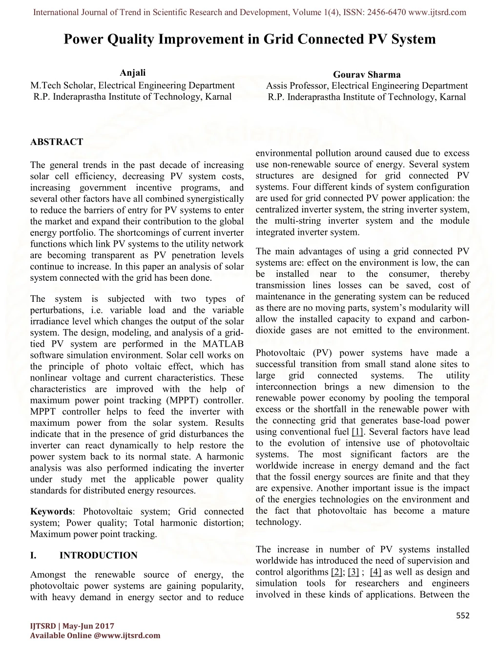
The general trends in the past decade of increasing solar cell efficiency, decreasing PV system costs, increasing government incentive programs, and several other factors have all combined synergistically to reduce the barriers of entry for PV systems to enter the market and expand their contribution to the global energy portfolio. The shortcomings of current inverter functions which link PV systems to the utility network are becoming transparent as PV penetration levels continue to increase. In this paper an analysis of solar system connected with the grid has been done. The system is subjected with two types of perturbations, i.e. variable load and the variable irradiance level which changes the output of the solar system. The design, modeling, and analysis of a grid tied PV system are performed in the MATLAB software simulation environment. Solar cell works on the principle of photo voltaic effect, which has nonlinear voltage and current characteristics. These characteristics are improved with the help of maximum power point tracking MPPT controller. MPPT controller helps to feed the inverter with maximum power from the solar system. Results indicate that in the presence of grid disturbances the inverter can react dynamically to help restore the power system back to its normal state. A harmonic analysis was also performed indicating the inverter under study met the applicable power quality standards for distributed energy resources Anjali | Gourav Sharma "Power Quality Improvement in Grid Connected PV System" Published in International Journal of Trend in Scientific Research and Development (ijtsrd), ISSN: 2456-6470, Volume-1 | Issue-4 , June 2017, URL: https://www.ijtsrd.com/papers/ijtsrd2196.pdf Paper URL: http://www.ijtsrd.com/engineering/electrical-engineering/2196/power-quality-improvement-in-grid-connected-pv-system/anjali<br>

E N D
International Journal of Trend in Scientific Research and Development, Volume 1(4), ISSN: 2456-6470 www.ijtsrd.com Power Quality Improvement in Grid Connected PV System Anjali Gourav Sharma M.Tech Scholar, Electrical Engineering Department R.P. Inderaprastha Institute of Technology, Karnal Assis Professor, Electrical Engineering Department R.P. Inderaprastha Institute of Technology, Karnal ABSTRACT The general trends in the past decade of increasing solar cell efficiency, decreasing PV system costs, increasing government incentive programs, and several other factors have all combined synergistically to reduce the barriers of entry for PV systems to enter the market and expand their contribution to the global energy portfolio. The shortcomings of current inverter functions which link PV systems to the utility network are becoming transparent as PV penetration levels continue to increase. In this paper an analysis of solar system connected with the grid has been done. environmental pollution around caused due to excess use non-renewable source of energy. Several system structures are designed for grid connected PV systems. Four different kinds of system configuration are used for grid connected PV power application: the centralized inverter system, the string inverter system, the multi-string inverter system and the module integrated inverter system. The main advantages of using a grid connected PV systems are: effect on the environment is low, the can be installed near to the consumer, thereby transmission lines losses can be saved, cost of maintenance in the generating system can be reduced as there are no moving parts, system’s modularity will allow the installed capacity to expand and carbon- dioxide gases are not emitted to the environment. Photovoltaic (PV) power systems have made a successful transition from small stand alone sites to large grid connected interconnection brings a new dimension to the renewable power economy by pooling the temporal excess or the shortfall in the renewable power with the connecting grid that generates base-load power using conventional fuel [1]. Several factors have lead to the evolution of intensive use of photovoltaic systems. The most significant factors are the worldwide increase in energy demand and the fact that the fossil energy sources are finite and that they are expensive. Another important issue is the impact of the energies technologies on the environment and the fact that photovoltaic has become a mature technology. The system is subjected with two types of perturbations, i.e. variable load and the variable irradiance level which changes the output of the solar system. The design, modeling, and analysis of a grid- tied PV system are performed in the MATLAB software simulation environment. Solar cell works on the principle of photo voltaic effect, which has nonlinear voltage and current characteristics. These characteristics are improved with the help of maximum power point tracking (MPPT) controller. MPPT controller helps to feed the inverter with maximum power from the solar system. Results indicate that in the presence of grid disturbances the inverter can react dynamically to help restore the power system back to its normal state. A harmonic analysis was also performed indicating the inverter under study met the applicable power quality standards for distributed energy resources. systems. The utility Keywords: Photovoltaic system; Grid connected system; Power quality; Total harmonic distortion; Maximum power point tracking. The increase in number of PV systems installed worldwide has introduced the need of supervision and control algorithms [2]; [3] ; [4] as well as design and simulation tools for researchers and engineers involved in these kinds of applications. Between the I. INTRODUCTION Amongst the renewable source of energy, the photovoltaic power systems are gaining popularity, with heavy demand in energy sector and to reduce 552 IJTSRD | May-Jun 2017 Available Online @www.ijtsrd.com
International Journal of Trend in Scientific Research and Development, Volume 1(4), ISSN: 2456-6470 www.ijtsrd.com different approaches for PV system design and simulation existing nowadays [5] ; [6], most popular tools are specific commercial software helping in design of PV systems like PVsol [7] and PVsyst [8]. These tools give a good approach of the PV system design and behavior in different conditions of work, but when a more detailed simulation is needed to a deep understand of the different components involved in the whole system these tools are not powerful enough. More powerful approaches have been developed using different commercial software for technical and engineering Pspice [9]; [10] ; [11] or MATLAB [12]; [13]; [14]; [15] ; [16]. As it is well known, there are currently various photovoltaic technologies on the market. The characteristics parameters of PV modules, usually given by the manufacturer, never are the same in real condition of operation. The evaluation of these parameters in real conditions of work is essential for a good modeling and accurate simulation of PV systems. On the other hand, the produced DC energy is altered by the power conditioning units which consist of MPP tracker and DC/AC converter. I= Output current of the PV cell. Iph= Cell generated current. Id= Diode current. Ish= Current drawn by shunt resistance. Ki=short (0.0032A/k(approx...)) circuit temp coefficient of cell T=module operating temperature in Kelvin. applications as Tr=reference temperature in kelvin=298k Q=charge of electron=1.9 ∗ 10−19 S=module irradiance (/m2) K=Boltzmann constant=1.38 ∗ 10−23 The important parameters of solar cell are open circuit voltage (Voc), short circuit current (Isc), Maximum Output power (Pmax). Equivalent Circuit Here it is assumed that the source current or the solar cell current which is of nearly constant. Id is the diode current, Diode is placed in parallel to ground the cells which are which are affected by the unshaded portion of the sun irradiation. Rsh is to represent the leakage current that is presented in the cell which is the order of 1000 ohms. Rse is the series resistance to replace the losses presents the cell. Vo is the output voltage or the open circuit voltage presented, at the terminals of the cell. Io is the current available at the output of the cell. The equivalent circuit of the solar cell is shown as below. II. Solar cell can be modelled as current source (Iph) in parallel with Diode (D), Shunt resistance (Rsh) and series resistance (Rse).Current and voltage profile of the solar cell depends on Atmosphere temperature (T), and irradiance (S). The output power of Photo voltaic cell is given by P=V*I. The current produced by the PV cell is equal to the current produced by the current source minus the diode and shunt resistance current. The light generated current of Photo voltaic cell depends on the solar irradiation and the temperature. MODELLING OF PV SYSTEM The equivalent circuit diagram of solar cell is shown in fig.1. The source current generated the cell is constant, as and when the temperature are constant. As the current generated by the cell depends on the temperature and the solar irradiation. (1) I Iph Id Ish S (2) Iph [ ISC Ki * ( T Tr )] * 1000 q ( v i * Rs (3) ) 1 AKT Id Io ( e 1 1 * q * Eg * Tr T 3 T (4) A K Io Ior * * e Tr 553 IJTSRD | May-Jun 2017 Available Online @www.ijtsrd.com
International Journal of Trend in Scientific Research and Development, Volume 1( International Journal of Trend in Scientific Research and Development, Volume 1(4), ISSN: 2456 2456-6470 www.ijtsrd.com The point at which maximum value of current and voltage are obtained is known as maximum power The point at which maximum value of current and voltage are obtained is known as maximum power point. RS I + ID ISH The maximum power point can be obtained by using The maximum power point can be obtained by using the fallowing methods. RSH V IL 1.Incremental conductance method 2.Perturb and observe method. 3.Constant voltage method 4.Constant current method 5.Fuzzy logic controller method. Here in this work, perturb and observe method is used. Incremental conductance method Perturb and observe method. - Fig.1. Equivalent circuit of a solar cell Fig.1. Equivalent circuit of a solar cell Fuzzy logic controller method. The diode current has the steeply increasing characteristics, with the voltage. The output current is the combination of cell current and the diode current, it results in the nonlinear characteristics of the output current and the voltage. The diode current has the steeply increasing output current is Here in this work, perturb and observe method is the combination of cell current and the diode current, it results in the nonlinear characteristics of the output In the perturb and observe method directly power is measured using voltage and current sensors. The power is calculated from the voltage and current values at Nth instant. By incrementing the values of duty cycle by a small ratio the voltage and current values will be measured at N+1th instant. The power value at Nth instant and N+1th instant will be compared. If the change in the power with respect to the is positive then the process is going in the correct direction, that is the positive direction. The duty cycle will be increased by a small ratio and the process will be continued for the next cycle. If the power with negative then the process is going after the maximum power in the negative direction. In that case the duty cycle will be decreased and the In the perturb and observe method directly power is measured using voltage and current sensors. The power is calculated from the voltage values at Nth instant. By incrementing the values of duty cycle by a small ratio the voltage and current values will be measured at N+1th instant. The power value at Nth instant and N+1th instant will be compared. If the change in the power wit the is positive then the process is going in the correct direction, that is the positive direction. The duty cycle will be increased by a small ratio and the process will be continued for the next cycle. If the power with respect to voltage is negative then the process is going after the maximum power in the negative direction. In that case the duty cycle will be decreased and the values will be updated for the next operation. values will be updated for the next operation. III. The efficiency of solar cell is low, in order to increase the efficiency maximum power tracking algorithms are used, for getting maximum possible power from the varying source. In photo voltaic power generation the I-V characteristics are non-linear, there feeding power to a certain load. This can be improved by using Boost converter whose duty cycle is controlled by using MPPT algorithm. MPPT FOR PV SYSTEM The efficiency of solar cell is low, in order to increase power tracking algorithms are used, for getting maximum possible power from the varying source. In photo voltaic power generation linear, there feeding power to a certain load. This can be improved by hose duty cycle is controlled The I-V,P-V characteristics the solar cell are shown as the figure 2 below, which are non linear in nature. The power is zero at the starting and at the final value of the curve. Because the non occurr maximum current and voltage at a same point, so as to maintain the operating point at a maximum power value a specially designed technique is required that is maximum power point technique. V characteristics the solar cell are shown as the figure 2 below, which are non linear in nature. The power is zero at the starting and at the final value of the curve. Because the non occurrence of the maximum current and voltage at a same point, so as to maintain the operating point at a maximum power value a specially designed technique is required that is dP , Then the slope of the characteristics is zer , Then the slope of the characteristics is zero. 0 dV The operation is taking place at the maximum point. Then no correction is required, the power supplied from the cell is the maximum value. supplied from the cell is the maximum value. The operation is taking place at the maximum power point. Then no correction is required, the power dP The slope of the characteristic is positive, for The slope of the characteristic is positive, for 0 dV getting maximum power operation the the converter will be increased, and the values of the voltage and current will be measured. The slope will be measured at the next cycles. be measured at the next cycles. getting maximum power operation the duty cycle of the converter will be increased, and the values of the voltage and current will be measured. The slope will dP , Then the slope of the characteristics is Then the slope of the characteristics is 0 dV negative. It is operating at a point power point. For getting the maximum power operation the duty cycle of the converter will be decreased. And the voltage and the current values will be measured from them the power will be calculated, be measured from them the power will be calculated, negative. It is operating at a point after the maximum power point. For getting the maximum power operation the duty cycle of the converter will be decreased. And the voltage and the current values will Fig. 2. I-V, P-V characteristics of the PV ce V characteristics of the PV cell. 554 IJTSRD | May-Jun 2017 Available Online @www.ijtsrd.com
International Journal of Trend in Scientific Research and Development, Volume 1( International Journal of Trend in Scientific Research and Development, Volume 1(4), ISSN: 2456 2456-6470 www.ijtsrd.com and this power will be compared with t value, this process will be continued for the next cycles. and this power will be compared with the previous value, this process will be continued for the next The simulation is done for the two seconds and divided in the two parts of one second each. In the first part the irradiation level is changed. From the time 0 sec.-0.3 sec the irradiance level is 600 KW/m from time 0.3 sec. to 0.5 sec. it is 700 KW/m 0.5 to 0.6 it is 800 KW/m2and from time 0.6 sec. to 2.0 sec. the irradiance level is 1000 KW/m 2.0 sec. the irradiance level is 1000 KW/m2. The simulation is done for the two seconds and divided in the two parts of one second each. In the first part the irradiation level is changed. From the 0.3 sec the irradiance level is 600 KW/m2, 0.3 sec. to 0.5 sec. it is 700 KW/m2 , from IV. This section gives the simulation MATLAB results about the work that has been proposed. It gives the results about the photovoltaic characteristics and the dependence of the results on the atmosphere conditions like temperature and irradiance. of the boost converter applying maximum power tracking technique, involving input and output voltage from the converter. It describes about the results relating to linear and nonlinear loads after applying P&O method of MPPT to the inverter and gives the results about the total harmonic results level. results about the total harmonic results level. SIMULATION AND RESULTS SIMULATION AND RESULTS This section gives the simulation MATLAB results about the work that has been proposed. It gives the results about the photovoltaic characteristics and the ence of the results on the atmosphere conditions like temperature and irradiance. The results of the boost converter applying maximum power tracking technique, involving input and output voltage from the converter. It describes about the results to linear and nonlinear loads after applying P&O method of MPPT to the inverter and gives the and from time 0.6 sec. to For the second case the value of the three phase load is change in the second part of the simulation i.e. at .5 second and load is made double (14.65 KW to 25.95 KW). The system is again checked for For the second case the value of the three phase load is change in the second part of the simulation i.e. at time 1.5 second and load is made double (14.65 KW to 25.95 KW). The system is again checked for another two cases, these are: 1.Minimum irradiance level and maximum load. 2.Maximum irradiance level and minimum load. Maximum irradiance level and minimum load. Minimum irradiance level and maximum load. 1. Change in irradiance level and Load As mentioned above the irradiance level is varied at time 0.3 sec, 0.5 and 0.6 sec and load at 1.5 sec. The various results obtained are shown in the following waveforms. Change in irradiance level and Load above the irradiance level is varied at time 0.3 sec, 0.5 and 0.6 sec and load at 1.5 sec. The various results obtained are shown in the following The grid connected PV system is subjected to different perturbances such as continuously variable load and variable irradiance level. In this work the system is studied under these two perturbances. The two cases are formed to analyze the system performance, these are: The grid connected PV system is subjected to different perturbances such as continuously variable e irradiance level. In this work the system is studied under these two perturbances. The two cases are formed to analyze the system 1.Change in irradiance level. 2.Change in the value of three phase load. Change in the value of three phase load. Fig.4. Irradiance level Fig.4. Irradiance level The irradiance level is changed as shown in the figure. From time 0.0 to 0.3 sec irradiance value is 600 KW/m2. The between time 0.3 to0.5 sec. it is 700 KW/m2 , between time 0.5 to 0.6 sec. it is 800KW/m2 and between time 0.6 to 2 sec. it is 1000 KW/m2. and between time 0.6 to 2 sec. it is 1000 KW/m2. The irradiance level is changed as shown in the figure. 0.3 sec irradiance value is 600 KW/m2. The between time 0.3 to0.5 sec. it is 700 KW/m2 , between time 0.5 to 0.6 sec. it is 800KW/m2 PQinv. PQinv. 2500 P-inverter Q-inverter 2000 1500 1000 500 0 -500 -1000 -1500 -2000 -2500 0 0.2 0.4 0.6 0.8 1 1.2 1.4 1.6 1.8 2 Time (Sec) Time (Sec) Offset=0 Fig. 5. Source active and reactive power. Fig. 5. Source active and reactive power. Fig.3. Flow chart of Perturb & Observe method of MPPT. of Perturb & Observe method of 555 IJTSRD | May-Jun 2017 Available Online @www.ijtsrd.com
International Journal of Trend in Scientific Research and Development, Volume 1(4), ISSN: 2456-6470 www.ijtsrd.com Vdc 180 160 140 120 100 Vdc (V) 80 60 40 20 0 -20 0 0.2 0.4 0.6 0.8 1 1.2 1.4 1.6 1.8 2 Time (Sec) Offset=0 Fig. 6 VDC Boost converter. Fig. 9. THD analysis of grid connected PV system. VDC Boost converter voltage should be constant with any perturbances to maintain the output voltage constant. Fig. 6 shows the VDC Boost converter output voltage waveform. As from the waveform it is seen that there is no change in the VDC Boost converter with irradiance level change and load change. Fig. 9. shows the THD found in the system and it is to be 3.77%, which is well below the 5% prescribed limit. V. This work gives the modeling and simulation of grid connected solar power system and the output voltage and current, output power versus voltage are observed at different irradiance and load conditions. The maximum power variation with the parameters are observed. The MPPT techniques for photovoltaic cells are developed and the output characterstics are observed at different irradiance level are observed. The boost converter applying the maximum power point technique based on P&O method is explained. The operation of boost converter at different operating conditions like turn on and turn off conditions are observed. The input and output voltages applied for the boost converter are shown and its importance is explained. The combination of boost converter with maximum power point tracking controller makes the converter to obtain the maximum power from solar cell. The operation of the inverter is explained with its different operating modes are the graphs for current- voltage and power to voltage are observed under different methods. Conclusions For the second part of the simulation the load is varied at time 1.5 sec. As the load increases the value of three phase current also increases accordingly to meet the load requirement. Fig. 7 shows the waveform of the three phase current drawn from the grid and it is doubled when the load is increased twice at time 1.5 sec. Iabc 600 400 Three Phase grid current 200 0 -200 -400 -600 Time (Sec) Fig.7. Three phase grid current. PQSource 104 2.5 P-source Q-source 2 Active and Reactive power 1.5 1 0.5 The comparison is carried out between different cases. The THD analysis is made for the two cases when the irradiance level is low and load is high and vice-versa. It is found that when irradiance level increases the penetration level of the PV system also increases. 0 Time (Sec) Fig. 8. Source active and reactive power. The power drawn from the grid is also increased at time 1.5 sec. and it can be seen from the fig. 8. Reactive power is constant as the load is purely active. 556 IJTSRD | May-Jun 2017 Available Online @www.ijtsrd.com
International Journal of Trend in Scientific Research and Development, Volume 1(4), ISSN: 2456-6470 www.ijtsrd.com References [11]S. Silvestre, A. Boronat, A. Chouder, “Study of bypass diodes configuration on PV modules”, Applied Energy 86 (9) (2009) 1632–1640. [12]http://www.mathworks.com/ [13]Geoff Walker, “Evaluating MPPT converter topologies using a MATLAB PV model”, Journal of Electrical & Electronics Engineering Australia 21 (1) (2001) 49–5 [14]Chao Shen, Ya-Ling He, Ying-Wen Liu, Wen- Quan Tao, “Modelling and simulation of solar radiation data processing Simulation Modelling Practice and Theory 16 (7) (2008) 721–735. [15]E. Román, R. Alonso, Elorduizapatarietxe, D. Goitia, “Intelligent PV module for grid-connected PV systems”, IEEE Transactions on Industrial Electronics 53 (4) (2006) 1066–1073. [16]Xiao-Qiang Guo, Wei-Yang Wu, He-Rong Gu, “Modeling and simulation of direct output current control for LCL-interfaced inverters with parallel Simulation Modelling Practice and Theory 18 (2010) 946–956 [1]S. Massoud, B. Wollenberg, “Toward a smart grid: power delivery for the 21st Century”, IEEE Power and Energy Magazine 3 (5) (2005) 34–41. [2]A. Chouder, S. Silvestre, “Automatic supervision and fault detection of PV systems based on power losses analysis”, Energy Management 51 (2010) 1929–1937. [3]S.K. Firth, K.J. Lomas, S.J. Rees, “A simple model of PV system performance and its use in fault detection”, Solar Energy 84 (2010) 624–635. [4]Syafaruddin, Engin Karatepe, Takashi Hiyama, “Polar coordinated fuzzy controller based real- time maximum-power photovoltaic system”, Renewable Energy 34 (2009) 2597–2606. [5]S. Silvestre, “Review of system design and sizing simulation tools”, in: T. Markvart, L. Castañer (Eds.), Practical Handbook of Photovoltaics, Fundamentals and Applications, Elsevier, Oxford, 2003, pp. 544–561. [6]Esfandyar Mazhari, Jiayun Zhao, Nurcin Celik, Seungho Lee, Young-Jun Son, Larry Head, “Hybrid simulation and optimization-based design and operation of generation, storage units, and grid”, Simulation Modelling Practice and Theory 19 (2011) 463– 481. [7]http://valentin- software.com/xcartgold/Photovoltaics/. [8]http://www.pvsyst.com/. [9]http://www.cadence.com/products/orcad/pspice_si mulation/pages/default.aspx. [10]L. Castañer, S. Silvestre, “Modelling PV Systems Using Pspice”, Wiley, Chichester, 2002. Conversion and with Simulink”, P. Ibañez, S. point control of grid-connected passive damping”, integrated photovoltaic 557 IJTSRD | May-Jun 2017 Available Online @www.ijtsrd.com