Download
1 / 57
580 likes | 771 Views
Tropical (Cyclone) Applications of Satellite Data. Andrea Schumacher Cooperative Institute for Research in the Atmosphere (CIRA) Fort Collins, Colorado Mark DeMaria NESDIS Center for Satellite Applications and Research (StAR) Regional and Mesoscale Meteorology Branch Fort Collins, Colorado

E N D
Tropical (Cyclone) Applications of Satellite Data Andrea Schumacher Cooperative Institute for Research in the Atmosphere (CIRA) Fort Collins, Colorado Mark DeMaria NESDIS Center for Satellite Applications and Research (StAR) Regional and Mesoscale Meteorology Branch Fort Collins, Colorado COMET Faculty Course August 10, 2010
Application: Track Forecasting • Initial position/storm structure analysis • Improvement of numerical models • Assimilation of satellite data • “Evaluation” of numerical models • Synoptic feature identification for qualitative prediction • Model analysis/satellite loop overlays provide assessment of t=0 hr accuracy
Center Fixing • Accurate positions necessary for estimation of storm motion • Animation of imagery • Visible/IR during day • GOES IR window and shortwave IR at night • Microwave imagery (SSM/I and AMSU-B) • Formal center fixes began in 2003
Storms with eyes are easiest… but still can have errors due to parallax
Storms without an eye more difficult Tropical Storm Lee 2005 Example of the Utility of 3.9 m (GOES Channel 2) data 10.7 m 3.9 m Helps to use combination of of satellite data types
Multi-Spectral Views of Hurricane Katrina(from www.nrlmry.navy.mil/tc_pages/tc_home.html) Visible GOES Microwave: DMSP SSMI 85 Ghz/H IR (10.7 m) GOES QuikSCAT Ocean Surface Winds
MODIS IR and water vapor winds GMS, Meteosat, and GOES cloud drift IR and visible winds GOES water vapor cloud top winds SSM/I wind speeds SSM/I precipitation estimates TRMM TMI precipitation estimates NOAA-17 HIRS 1b radiances AQUA AIRS 1b radiances NOAA-15, NOAA-16, NOAA-18 and AQUA AMSU-A 1b radiance NOAA-15, -16, and -17 AMSU-B 1b radiances GOES-12 5x5 cloud cleared radiances NOAA-16 and -17 SBUV ozone profiles Satellite data used in NCEP’soperational data assimilation systems Satellite data also used to help estimate initial storm position, motion, intensity and wind structure for “TC Vitals” file used to initialize regional models
Classification of Satellite Input • Satellite Radiances (IR and microwave sounders) • T , water vapor and trace gas (e.g. ozone) profiles • Indirect impact on wind through assimilation • Satellite winds • Feature track winds • Scatterometer surface winds (ASCAT and Windsat) • Satellite precipitation and TPW estimates • Model moisture condensate variables • Land and sea surface properties • Boundary conditions and atmosphere-ocean interface variables • Satellite altimetry • Sub-surface ocean structure
Satellite Wind Measurements:Feature Tracking Methods • Track features in imagery • Measures total wind component • Height assignment is necessary • Winds are layer averages • Views sometimes blocked by clouds • Higher resolution with GOES RSO
Impact of Removing Satellite Dataon NCEP GFS Track Forecasts
Model “Evaluation” Overlay of NCEP Global Model Analysis and Water Vapor Imagery - Check for Consistency of Synoptic Features- 300 mb GFS Winds and WV Imagery 8 Nov 2008, Hurricane Paloma
Application: Intensity Forecasting • Less skillful than track forecasts • Intensity change sensitive to wide range of physical processes • eyewall and other convection • boundary layer and air-sea interaction • microphysical processes • synoptic scale interaction • ocean interaction • Numerical forecasts often inaccurate • Greater reliance on extrapolation, empirical and statistical forecast methods
Intensity Forecasting (cont…) • Intensity monitoring • Dvorak method • AMSU method • Detection of intensity trends • Storm relative, time average IR loops • Microwave data to identify concentric eye structure • Qualitative analysis of storm environment • Improved SST analysis • Ocean altimetry data (heat content) • Quantitative use in statistical models • Wind structure analysis
Overview of the Dvorak Technique • Visible and Infrared Techniques • Uses patterns and measurements as seen on satellite imagery to assign a number (T number) representative of the cyclone’s strength. • The T number scale runs from 0 to 8 in increments of 0.5.
Patterns of Visible Dvorak Technique 1. Curved Band 2. Shear Pattern 3. CDO 4. Eye 4a. Banded Eye
Infrared (IR) Technique • Can be used during night as well as during day • At times more objective than visible technique
Example Digital IR: Hurricane Erika 1515 UTC 8 September 1997 • Warmest eye pixel 16 °C • Warmest pixel 30 nmi (55 km) from center -57 °C • Nomogram gives Eye no. =5.8 or close to 6
Uncorrected Corrected AMSU-A Temperature/Gradient Wind Retrievals(Demuth et al 2006, JAM) T(r,z) Ps(x,y) V(r,z)
AMSU Predicted vs. Observed Maximum Winds (Statistical relationships between AMSU retrievals and Intensity) Single or multiple channel methods also developed by Brueske et al 2003 And Spencer and Braswell 2001
Intensity Trends Visible Imagery Loop 9/21/98 19:02 to 20:10Hurricane Georges During Rapid Intensification
Animation of 6-hr Motion- Relative IR Average Images(Averaging helps separate short/long term intensity changes) • Loop 1 – just prior to onset of Mitch’s rapid intensification • Loop 2 – during Mitch’s rapid intensification
Environmental Interactions • Vertical Shear of Horizontal Wind • Limits intensification • Prevents establishment of vertically aligned circulation • Increases ventilation of eyewall circulation • Trough Interaction • Sometimes leads to intensification • Positive momentum flux convergence in upper levels • Increases vertical depth of cyclonic flow • Possible trigger of eye-wall cycle
8-Frame Water Vapor Imagery Loop 9/20/98 23:45 to 9/21/98 23:45Hurricane/Trough Interaction
Improved Sea Surface Temperature • SST has strong • influence on • intensity Change • Geo and Polar • data used in SST • products • Multi-sensor • approach • to correct for • aerosol effects
Ocean Heat Content Retrievals from Satellite Altimetry
Statistical Intensity Forecast Improvements Using Satellite Data(RAMM Branch Joint Hurricane Testbed Project) • Goal: To determine if satellite data (GOES and satellite altimetry) can improve the intensity forecasts from the statistical-dynamical SHIPS model • Method: Parallel version of SHIPS with satellite input was run in real-time for 2002-03 • Satellite SHIPS made operational in 2004 • Evaluation: Compare operational and parallel SHIPS forecasts for Atlantic and east Pacific
Input from GOES Imagery and OHC Analysis Hurricane Floyd 14 Sept 1999 OHC 26 Sept 2002
SHIPS Model Improvements with Satellite Input(2002-2003 Experimental Forecasts)
Impact on SHIPS Forecasts for Category 5 Storms since OHC was added • Isabel (03), Ivan (04), Emily, Katrina, Rita, Wilma (05) • Verify only over-water part of forecast
Application: Wind Structure • Operational requirement for radii of 34, 50 and 64 kt surface winds • Satellite techniques • Feature tracked winds for outer circulation • SSM/I surface wind speeds • Scatterometer observations (ASCAT, former QuikSCAT • AMSU-A wind nonlinear balance retrievals • Empirical relationships with IR data • Experimental, K. Mueller MS Thesis
Properties of Satellite Winds for TC Analysis • IR/WV/Vis cloud drift winds • High quality, but far from the center • Spatial coverage often limited • Height assignment errors • ASCAT (active)– surface wind vectors • Speeds good to ~50 kts • Rainfall effects winds • Directions sometimes unreliable • Windsat (passive) - surface wind vectors • Properties similar to ASCAT • SSM/I surface wind speeds • Rain free areas • Speed only • AMSU nonlinear balance winds • Temporal coverage limited • Not at the surface • Can not resolve inner core due to 50 km resolution
x Cloud drift and water vapor winds Hurricane Ivan 12 Sept 2004 From CIMSS
QuikSCAT and AMSU Nonlinear Balance Winds for Hurricane Ivan QSCAT ( Plot provided by Remote Sensing Systems available at www.remss.com )
SSM/I Wind Speeds for Hurricane Ivan (Plot provided by Remote Sensing Systems available at www.remss.com )
Hurricane FLOYD – 1515 UTC 14 Sep 99 Hurricane IRIS – 0015 UTC 9 Oct 01
Inner Core TC Winds from IR Imagery(Mueller et al 2007, WF) • Model wind field by sum of storm motion and symmetric • Assume Vmis know from Dvorak or other methods • Estimate x and Rm from IR imagery, Vm and latitude Vm=100 kts, Rm=55 km, x=0.5
Experimental RAMMB Product Satellite-Only Wind analysis • Combine all available satellite inputs in variation analysis • Find Uij Vij to minimize cost function C: C = wk[(uk-Uk)2 + (vk-Vk)2] + wm(sm-Sm)2 + [(rUij2 +rVij2) + (Uij2 + Vij2] • Uij Vij are gridded radial and tangential wind • u k,vk = obs, Uk Vk= model counterpart of ukvk • sm,Sm are observed wind speeds and model counterpart • Wk andWm are data weights • , terms are smoothness constraints • For wind analysis, “model” is gridded function interpolated to observation point • azimuthal smoothing >> radial smoothing • Based on Thacker and Long (1990) • Could also add other constraints if necessary
Example: Hurricane Ivan 0912 18Z R34 175 180 125 185 R50 120 115 80 125 R64 80 65 60 60 R34 150 120 100 150 R50 100 90 70 90 R64 80 60 45 55 From satellite analysis From NHC 18Z advisory http://rammb.cira.colostate.edu/products/tc_realtime/
Application: Hurricane Rainfall Forecasting • Majority of recent U.S. loss of life from tropical cyclones from inland flooding • Except for Katrina (2005) • Forecast accuracy not well documented • Evaluation in progress • Forecast methods • Rule of thumb: STR=100/c • Numerical models: NAM, GFS, GFDL • Rainfall rate estimates from IR/microwave (QPE) • Satellite rainfall forecasts (QPF) • Extrapolation of QPE • Rainfall CLIPER model
Rainfall Estimation From GOES Hydro-Estimator> <Multi-Spectral
QPE/QPF Forecast Examples: TC 02W and TC 26S, 9 April 2003 SSM/I Rainfall Rate AMSU Rainfall Rate 26S 02W Extrapolated SSM/I Rainfall Extrapolated AMSU Rainfall 02W 26S
Application: Formation (Genesis) Total Precipitable Water RAMMB TC Formation Probability Product http://rammb.cira.colostate.edu/projects/gparm/gparm_glob_test/ http://rammb.cira.colostate.edu/ramsdis/online/tropical.asp