Download
1 / 38
390 likes | 576 Views
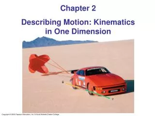
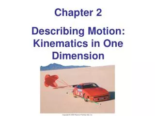
Chapter 2 Kinematics in One Dimension. Chapter Goal: To learn how to solve problems about motion in a straight line. Slide 2-2. Chapter 2 Preview. Kinematics is the name for the mathematical description of motion.

E N D
Chapter 2 Kinematics in One Dimension Chapter Goal: To learn how to solve problems about motion in a straight line. Slide 2-2
Chapter 2 Preview • Kinematics is the name for the mathematical description of motion. • This chapter deals with motion along a straight line, i.e., runners, rockets, skiers. • The motion of an object is described by its position, velocity, and acceleration. • In one dimension, these quantities are represented by x,vx,and ax. • You learned to show these on motion diagrams in Chapter 1. Slide 2-3
Uniform Motion • If you drive your car at a perfectly steady 60 mph, this means you change your position by 60 miles for every time interval of 1 hour. • Uniform motion is when equal displacements occur during any successive equal-time intervals. • Uniform motion is always along a straight line. Riding steadily over level ground is a good example of uniform motion. Slide 2-20
Uniform Motion • An object’s motion is uniform if and only if its position-versus-time graph is a straight line. • The average velocity is the slope of the position-versus-time graph. • The SI units of velocity are m/s. Slide 2-21
Scalars and Vectors • The distance an object travels is a scalar quantity, independent of direction. • The displacement of an object is a vector quantity, equal to the final position minus the initial position. • An object’s speed v is scalar quantity, independent of direction. • Speed is how fast an object is going; it is always positive. • Velocity is a vector quantity that includes direction. • In one dimension the direction of velocity is specified by the or sign. Slide 2-28
Instantaneous Velocity • An object that is speeding up or slowing down is not in uniform motion. • In this case, the position-versus-time graph is not a straight line. • We can determine the average speed vavg between any two times separated by time interval t by finding the slope of the straight-line connection between the two points. • The instantaneous velocity is the object’s velocity at a single instant of time t. • The average velocity vavgs/t becomes a better and better approximation to the instantaneous velocity as t gets smaller and smaller. Slide 2-31
Instantaneous Velocity Motion diagrams and position graphs of an accelerating rocket. Slide 2-32
Instantaneous Velocity • As ∆t continues to get smaller, the average velocity vavg ∆s/∆t reaches a constant or limiting value. • The instantaneous velocity at time t is the average velocity during a time interval ∆t centered on t, as ∆t approaches zero. • In calculus, this is called the derivative of s with respect to t. • Graphically, ∆s/∆t is the slope of a straight line. • In the limit ∆t 0, the straight line is tangent to the curve. • The instantaneous velocity at time t is the slope of the line that is tangent to the position-versus-time graph at time t. Slide 2-33
A Little Calculus: Derivatives • ds/dt is called the derivative of s with respect to t. • ds/dt is the slope of the line that is tangent to the position-versus-time graph. • Consider a function u that depends on time as uctn, where c and n are constants: • The derivative of a constant is zero: • The derivative of a sum is the sum of the derivatives. If u and ware two separate functions of time, then: Slide 2-46
Derivative Example • Velocity is the derivative of s with respect to t: • The figure shows the particle’s position and velocity graphs. • The value of the velocity graph at any instant of time is the slope of the position graph at that same time. Suppose the position of a particle as a function of time is s = 2t2 m where t is in s. What is the particle’s velocity? Slide 2-47
Finding Position from Velocity • Suppose we know an object’s position to be si at an initial time ti. • We also know the velocity as a function of time between ti and some later time tf. • Even if the velocity is not constant, we can divide the motion into N steps in which it is approximately constant, and compute the final position as: • The curlicue symbol is called an integral. • The expression on the right is read, “the integral of vsdt from ti to tf.” Slide 2-54
Finding Position From Velocity • The integral may be interpreted graphically as the total area enclosed between the t-axis and the velocity curve. • The total displacement ∆sis called the “area under the curve.” Slide 2-55
A Little More Calculus: Integrals • Taking the derivative of a function is equivalent to finding the slope of a graph of the function. • Similarly, evaluating an integral is equivalent to finding the area under a graph of the function. • Consider a function u that depends on time as uctn, where c and n are constants: • The vertical bar in the third step means the integral evaluated at tf minus the integral evaluated at ti. • The integral of a sum is the sum of the integrals. If u and w are two separate functions of time, then: Slide 2-60
Motion with Constant Acceleration • The SI units of acceleration are (m/s)/s, or m/s2. • It is the rate of change of velocity and measures how quickly or slowly an object’s velocity changes. • The average acceleration during a time interval ∆t is: • Graphically, aavg is the slope of a straight-line velocity-versus-time graph. • If acceleration is constant, the acceleration as is the same as aavg. • Acceleration, like velocity, is a vector quantity and has both magnitude and direction. Slide 2-64
The Kinematic Equations of Constant Acceleration • Suppose we know an object’s velocity to be vis at an initial time ti. • We also know the object has a constant acceleration of as over the time interval ∆ttf − ti. • We can then find the object’s velocity at the later time tf as: Slide 2-81
The Kinematic Equations of Constant Acceleration • Suppose we know an object’s position to be siat an initial time ti. • It’s constant acceleration as is shown in graph (a). • The velocity-versus-time graph is shown in graph (b). • The final position sf is si plus the area under the curve of vs between ti and tf : Slide 2-82
The Kinematic Equations of Constant Acceleration • Suppose we know an object’s velocity to be vis at an initial position si. • We also know the object has a constant acceleration of as while it travels a total displacement of ∆ssf − si. • We can then find the object’s velocity at the final position sf: Slide 2-83
The Kinematic Equations of Constant Acceleration Motion with constant velocity and constant acceleration. These graphs assume si = 0, vis> 0, and (for constant acceleration) as> 0. Slide 2-85
Free Fall • The motion of an object moving under the influence of gravity only, and no other forces, is called free fall. • Two objects dropped from the same height will, if air resistance can be neglected, hit the ground at the same time and with the same speed. • Consequently, any two objects in free fall, regardless of their mass, have the same acceleration: In the absence of air resistance, any two objects fall at the same rate and hit the ground at the same time. The apple and feather seen here are falling in a vacuum. Slide 2-94
Free Fall • Figure (a) shows the motion diagram of an object that was released from rest and falls freely. • Figure (b) shows the object’s velocity graph. • The velocity graph is a straight line with a slope: • Where g is a positive number which is equal to 9.80 m/s2 on the surface of the earth. • Other planets have different values of g. Slide 2-95
Example 2.14 Finding the Height of a Leap Slide 2-98
Example 2.14 Finding the Height of a Leap Slide 2-99
Example 2.14 Finding the Height of a Leap Slide 2-100
Example 2.14 Finding the Height of a Leap Slide 2-101
Motion on an Inclined Plane • Figure (a) shows the motion diagram of an object sliding down a straight, frictionless inclined plane. • Figure (b) shows the the free-fall acceleration the object would have if the incline suddenly vanished. • This vector can be broken into two pieces: and . • The surface somehow “blocks” , so the one-dimensional acceleration along the incline is • The correct sign depends on the direction the ramp is tilted. Slide 2-102
Example 2.16 From Track to Graphs Slide 2-106
Example 2.16 From Track to Graphs Slide 2-107
Example 2.16 From Track to Graphs Slide 2-108
Example 2.16 From Track to Graphs Slide 2-109
Example 2.19 Finding Velocity from Acceleration Slide 2-114
Example 2.19 Finding Velocity from Acceleration Slide 2-115
Chapter 2 Summary Slides Slide 2-116
General Principles Slide 2-117
General Principles Slide 2-118
Important Concepts Slide 2-119
Important Concepts Slide 2-120