Download
1 / 24
290 likes | 570 Views
Interpolation Tools. Lesson 5 overview. Concepts Sampling methods Creating continuous surfaces Interpolation Density surfaces in GIS Interpolators IDW, Spline,Trend, Kriging,Natural neighbors TopoToRaster Assessing accuracy Exercise 5. Creating surfaces. Interpolate from sample points

E N D
Lesson 5 overview • Concepts • Sampling methods • Creating continuous surfaces • Interpolation • Density surfaces in GIS • Interpolators • IDW, Spline,Trend, Kriging,Natural neighbors • TopoToRaster • Assessing accuracy • Exercise 5
Creating surfaces • Interpolate from sample points • Example: Terrain, pH value, water quality • Convert from another format • Example: USGS Digital Elevation Model (DEM) • Four ways to represent surfaces:
Functional surface X,Y • Considered to be continuous • For an x,y location, only one z-value • NOT a true 3D model: 2 ½ dimensional • Can be used to represent: • Terrestrial surfaces • Statistical surfaces • Mathematical surfaces Z1 Z2 Z3
What is Interpolation? • Procedure to predict value at unsampled locations within sampled region • Based on the principle of spatial autocorrelation or spatial dependence • Spatial autocorrelation — measures degree of relationship/dependence between near and distant objects • Implements Tobler’s First law of Geography: “everything is related to everything else, but close things are closely related”
Elements of interpolation • The known points (samples) • Sample factors - size, Iimits, location ,outliers • The unknown points (interpolated values) • Interpolation models: • Deterministic - create surfaces from measured points, based on either the extent of similarity (IDW) or degree of smoothing (Trend). • Geostatistical - based on statistics (Kriging) with advanced prediction modeling, includes measure of certainty or accuracy of predictions. • Different interpolation methods will (almost always) produce different results.
Sampling a surface • Perfect surface requires infinite number of measurements • Therefore samples need to be significant and random, if possible • Error increases away from sample points
Linear interpolation • Interpolation of cell values • A best estimate between samples • May consider: • Distance • Weight • Used for: • Predicting • Forecasting • Describing • Understanding • Calculating • Estimating • Analyzing • Explaining Known Values 1 1.125 1.25 1.375 1.5 1.675 1.75 1.875 2 1 Mile
Controlling sample points for interpolation • IDW, Spline & Kriging support control of sample numbers • Sample methods: • Nearest neighbors — you choose how many • Search radius — variable or max distance • Returns NoData if insufficient samples
Barriers to interpolation • Barriers represented by line feature classes • Examples: Faults, cliffs, levees, depth to ground water • Restricts samples to same side of line as cell • IDW, KRIGING ()support barriers
Interpolating unknown values • Input • Point dataset • x,y coordinates in a text file • Output • Floating-point raster • Tools
Interpolation types • Deterministic or Geostatistical • Deterministic: • Surface created from samples based on extent of similarity or degree of smoothing. • E.g., IDW, Spline,Trend • Geostatistical • Spatial variation modeled by random process with spatial autocorrelation • Creates error surface — indication of prediction validity • E.g., Kriging
IDW • Deterministic Interpolation technique • Influence of known values diminishes with distance • Surface will not pass through samples (averaging) • Power value and barrier can be used • Sample subset defined by • Nearest neighbor • Fixed radius
lDW parameters • Best for dense evenly spaced samples • No estimates above max or below mm sample value • Can adjust relative influence or power of samples Z-Value Distance Power 1 Z-Value Power 2 Distance
Natural Neighbor Interpolation • Uses Thiessen polygon network of scatter points. • Interpolation by weighted average of surrounding or neighboring data points • Area-based weights • Cell value is “natural neighbor” of interpolation subset • Resulting surface analogous to a taut rubber sheet stretched to meet all the data. • Works well with clustered scatter points • Efficiently handles large numbers of input points
Spline • The surface passes exactly through the sample points • Fits a minimum-curvature surface through the input points • Like a rubber sheet that is bent around the samples • Best for smoothly varying surfaces (e.g., temperature) • Can predict ridges and valleys Z-Value Distance
Choosing a spline type • Regularized • A looser fit, but may have overshoots and undershoots • Generally makes a smoother surface • Higher values of {weight} smooth more • Tension • Forces the curve • Generally makes a coarser surface • Higher values of {weight} coarsen more than lower values Tension Regularized
Trend • Inexact interpolator: • Surface usually not through sample points • Detects trends in the sample data • Similar to natural phenomena, which usually vary smoothly. • Statistical approach: • Allows statistical significance of the surface and uncertainty of the predicted values to be calculated • Fits one polynomial equation to entire surface First order trend surface Order 1: No curve (flat tilted surface) 2: One curve 3: Two curves 4: Three curves, etc.
Kriging • A powerful statistical technique • Predicted values derived from measure of relationship in samples • Employs sophisticated weighted average technique • Cell value can exceed sample value range • Surface does not pass through samples • Various types of kriging • Uses a search radius • Fixed • Variable
Kriging methods • Several methods — spatial analyst supports: • Ordinary — assumes overall area mean; no trend. • Universal — assumes unknown trend in area mean. • Geostatistical analyst extension — supports more Z-Value Distance
Topo to Raster • Interpolates elevation imposing constraints to ensure: • Connected drainage structure. • Correct representation of ridges and streams from input data. • Deploys iterative finite difference interpolation technique. • Optimized to computational efficiency of ‘local’ interpolation without losing the surface continuity of global interpolation • Designed to work intelligently with contour inputs.
Visual comparisons of Interpolators IDW Spline Kriging Topo to Raster Natural Neighbor
Feature density estimation • Count occurrences of a phenomena within an area and distribute it through the area • Similar to focal functions • Performs statistics on features • Population field influences density • Use points or lines as input • Examples • Population per square kilometer • Road density per square mile • The number of customers per square mile
Testing your surface • Different interpolators will produce different results with same input data. • No single method is more accurate than others for all situations. • Accuracy — may be determined by comparison with a second set of “withheld” samples for accuracy checking. • Remove random test sample points • Create surface • Interpolate • Did interpolator predict missing samples? • Repeat • Try with each interpolator • Select the method based on knowledge of the the study area, phenomena of interest, and available resources.