Download
1 / 22
300 likes | 669 Views
Atomic Orbitals. SCH4U0 Tabone. Orbital Shapes. In previous lessons we alluded to the fact that the different orbitals (subshells) have their own distinct shapes Now we are going to discuss these shapes However, before we can do that we must discuss our views about electrons

E N D
Atomic Orbitals SCH4U0 Tabone
Orbital Shapes • In previous lessons we alluded to the fact that the different orbitals (subshells) have their own distinct shapes • Now we are going to discuss these shapes • However, before we can do that we must discuss our views about electrons • Typically we view them as particles • Now we view them as waves as well • How does this affect our model of the atom (in respect to orbitals)?
Heisenberg Uncertainty Principle • The Heisenberg Uncertainty Principle is a core foundation of quantum theory and greatly influences our view of electrons in orbitals • The principle states that the product of the uncertainty in position and momentum of a particle must be greater than a constant • There are a few important consequences of this
Heisenberg Uncertainty Principle • The more accurately we try to determine the position of a particle, the less accurately we know its momentum • We know where it IS but not where it is GOING • The more accurately we try to determine the momentum of a particle, the less accurately we know its position • We know where it is going and how fast it is moving, but not where it is • This can be illustrated fairly simply
Uncertainty • If we take a laser and pass it through a slit, we can continuously decrease the size of the slit • This will lower our uncertainty in the position of the photons • Eventually, as we continue to decrease our uncertainty in where the photons are, our uncertainty in their position must start to increase • This causes the beam to widen
What Does This Mean? • For us, this means that we have no accurate way of simultaneously knowing every property of the electrons in the atom • If we want to model the atom showing the exact positions and momentums of the electrons, we can’t • So how do we model the atom? • We use Schrödinger’s wave equation • Or at least a certain interpretation of it
Schrödinger’s Wave Equation • Schrödinger was able to make an equation that describes the position of all the electrons in an atom • It was based on the wave nature of matter • It is also extremely complicated to solve for any atom other than hydrogen
Schrödinger’s Wave Equation • What we need to know about this equation is how it is interpreted • The equation is viewed as representing all of the possible configurations (or states) the atom can be in • Each state is assigned a probability • The exact state in which an atom currently is can only be known through experiment • So we say that an atom has a probability of existing in any of the possible states at any given time, and we don’t really know which is true until we try and observe it
Schrödinger’s Cat • This can be illustrated using a simple setup with a cat in a box • This was first suggested as a thought experiment by Schrödinger to show why the probabilistic interpretation of his equation was incorrect • But in reality it underlines why the probabilistic interpretation works • The key point to remember is that radioactivity is a probabilistic quantum process • There is a finite chance that particles will “jump” out of the nucleus in a given increment of time
Schrödinger’s Cat Hammer Fuzzy Cat Geiger Counter Poisonous Gas Radioactive Material
Schrödinger’s Cat • There is a 50% chance the radioactive material will decay in 1 hour and a 50% chance that it will not • Meaning that at the end of the hour there is an equal chance that the cat is alive or dead – and we do not know which is true • So we say that at the hour mark the cat is both alive and the dead • The state condenses into one or the other when we open the box and make an observation
Electron Clouds • So what does this mean about electrons in atoms? • Since we cannot know where an electron is at any given time, we instead determine probable locations for the electron • We sum these probable locations up and view the electron instead as a cloud of electron density
Atomic Orbitals • If we analyze the electron clouds of different orbitals we can see that they all have characteristic shapes • s-orbitals
Atomic Orbitals • p-orbitals
Atomic Orbitals • d-orbitals
Electron Density Graphs • When electron density is graphed against distance from the nucleus, some interesting trends are seen • Orbitals of the same type have an increasing number of nodes as their energy level increases • 1s has no node, 2s has 1 node, 3s has 2 nodes, etc... • 2p has no node, 3p has 1 node, 4p has 2 nodes, etc... • A node is an area with little to no electron density
Electron Density Graphs Electron Density
Electron Density Graphs • Similarly, if we compare orbitals within the same energy level there is a pattern • As the ℓ number increases, the # of nodes decreases • 3s has 2 nodes, 3p has 1 nodes, 3d has 0 node • This same trend is shown in every energy level • The highest energy orbital always has 0 nodes
Quantum Tunnelling • Using the probabilistic approach to viewing matter, every particle has a probability of existing anywhere • But most of these probabilities are extremely small • This can be used however to transport particles through and across barriers • Ex: an alpha particle (helium nucleus) within a larger nucleus (like Ra) has a small probability of existing outside of the nucleus • This is how radioactive decay occurs Ra-226 Rn-222 + He
Quantum Tunnelling • Quantum tunnelling is also the phenomenon behind touch screens • The electrons in the screen have a small probability of being located in the sensors below the screen. • As the screen is pushed and the screen moves closer the sensors beneath, the probability increases • Eventually the probability is large enough that a significant (though small) number of electrons “jumps” from the screen to the sensors and starts an electric current