Download
1 / 1
10 likes | 118 Views
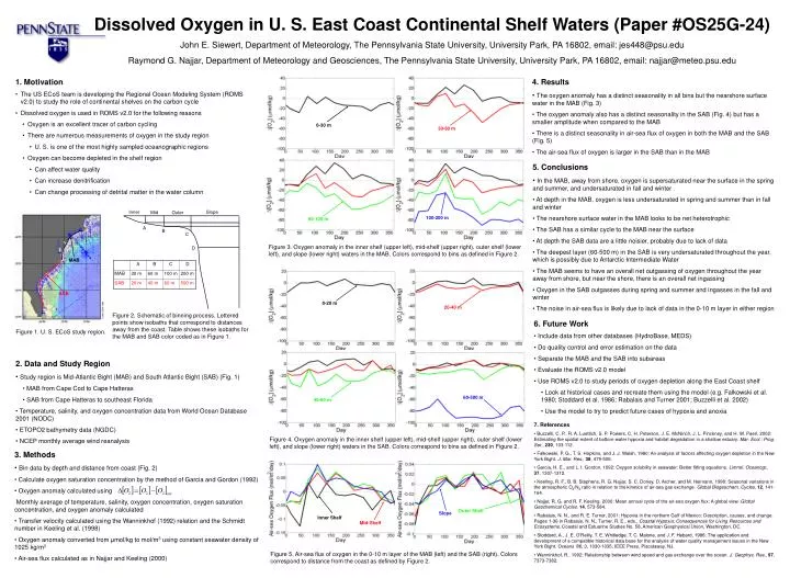
0-30 m. 30-60 m. Inner. Slope. Mid. Outer. 100-200 m. 60-100 m. A. B. C. MAB. D. SAB. 0-20 m. 20-40 m. 60-500 m. 40-60 m. Outer Shelf. Slope. Inner Shelf. Mid-Shelf. Dissolved Oxygen in U. S. East Coast Continental Shelf Waters (Paper #OS25G-24)

E N D
0-30 m 30-60 m Inner Slope Mid Outer 100-200 m 60-100 m A B C MAB D SAB 0-20 m 20-40 m 60-500 m 40-60 m Outer Shelf Slope Inner Shelf Mid-Shelf Dissolved Oxygen in U. S. East Coast Continental Shelf Waters (Paper #OS25G-24) John E. Siewert, Department of Meteorology, The Pennsylvania State University, University Park, PA 16802, email: jes448@psu.edu Raymond G. Najjar, Department of Meteorology and Geosciences, The Pennsylvania State University, University Park, PA 16802, email: najjar@meteo.psu.edu • Motivation • The US ECoS team is developing the Regional Ocean Modeling System (ROMS v2.0) to study the role of continental shelves on the carbon cycle • Dissolved oxygen is used in ROMS v2.0 for the following reasons • Oxygen is an excellent tracer of carbon cycling • There are numerous measurements of oxygen in the study region • U. S. is one of the most highly sampled oceanographic regions • Oxygen can become depleted in the shelf region • Can affect water quality • Can increase denitrification • Can change processing of detrital matter in the water column • 4. Results • The oxygen anomaly has a distinct seasonality in all bins but the nearshore surface water in the MAB (Fig. 3) • The oxygen anomaly also has a distinct seasonality in the SAB (Fig. 4) but has a smaller amplitude when compared to the MAB • There is a distinct seasonality in air-sea flux of oxygen in both the MAB and the SAB (Fig. 5) • The air-sea flux of oxygen is larger in the SAB than in the MAB • 5. Conclusions • In the MAB, away from shore, oxygen is supersaturated near the surface in the spring and summer, and undersaturated in fall and winter • At depth in the MAB, oxygen is less undersaturated in spring and summer than in fall and winter • The nearshore surface water in the MAB looks to be net heterotrophic • The SAB has a similar cycle to the MAB near the surface • At depth the SAB data are a little noisier, probably due to lack of data • The deepest layer (60-500 m) in the SAB is very undersaturated throughout the year, which is possibly due to Antarctic Intermediate Water • The MAB seems to have an overall net outgassing of oxygen throughout the year away from shore, but near the shore, there is an overall net ingassing • Oxygen in the SAB outgasses during spring and summer and ingasses in the fall and winter • The noise in air-sea flux is likely due to lack of data in the 0-10 m layer in either region Figure 3. Oxygen anomaly in the inner shelf (upper left), mid-shelf (upper right), outer shelf (lower left), and slope (lower right) waters in the MAB. Colors correspond to bins as defined in Figure 2. Figure 2. Schematic of binning process. Lettered points show isobaths that correspond to distances away from the coast. Table shows these isobaths for the MAB and SAB color coded as in Figure 1. • 6. Future Work • Include data from other databases (HydroBase, MEDS) • Do quality control and error estimation on the data • Separate the MAB and the SAB into subareas • Evaluate the ROMS v2.0 model • Use ROMS v2.0 to study periods of oxygen depletion along the East Coast shelf • Look at historical cases and recreate them using the model (e.g. Falkowski et al. 1980; Stoddard et al. 1986; Rabalais and Turner 2001; Buzzelli et al. 2002) • Use the model to try to predict future cases of hypoxia and anoxia Figure 1. U. S. ECoS study region. • 2. Data and Study Region • Study region is Mid-Atlantic Bight (MAB) and South Atlantic Bight (SAB) (Fig. 1) • MAB from Cape Cod to Cape Hatteras • SAB from Cape Hatteras to southeast Florida • Temperature, salinity, and oxygen concentration data from World Ocean Database 2001 (NODC) • ETOPO2 bathymetry data (NGDC) • NCEP monthly average wind reanalysis • 7. References • Buzzelli, C. P., R. A. Luettich, S. P. Powers, C. H. Peterson, J. E. McNinch, J. L. Pinckney, and H. W. Paerl, 2002: Estimating the spatial extent of bottom-water hypoxia and habitat degradation in a shallow estuary. Mar. Ecol.: Prog. Ser., 230, 103-112. • Falkowski, P. G., T. S. Hopkins, and J. J. Walsh, 1980: An analysis of factors affecting oxygen depletion in the New York Bight. J. Mar. Res., 38, 479-506. • Garcia, H. E., and L. I. Gordon, 1992: Oxygen solubility in seawater: Better fitting equations. Limnol. Oceanogr., 37, 1307-1312. • Keeling, R. F., B. B. Stephens, R. G. Najjar, S. C. Doney, D. Archer, and M. Heimann, 1998: Seasonal variations in the atmospheric O2/N2 ratio in relation to the kinetics of air-sea gas exchange. Global Biogeochem. Cycles, 12, 141-164. • Najjar, R. G. and R. F. Keeling, 2000: Mean annual cycle of the air-sea oxygen flux: A global view. Global Geochemical Cycles, 14, 573-584. • Rabalais, N. N., and R. E. Turner, 2001: Hypoxia in the northern Gulf of Mexico: Description, causes, and change. Pages 1-36 in Rabalais, N. N., Turner, R. E., eds., Coastal Hypoxia: Consequences for Living Resources and Ecosystems, Coastal and Estuarine Studies No. 58, American Geophysical Union, Washington, DC. • Stoddard, A., J. E. O’Reilly, T. E. Whitledge, T. C. Malone, and J. F. Hebard, 1986: The application and development of a compatible historical data base for the analysis of water quality management issues in the New York Bight. Oceans ’86, 3, 1030-1035, IEEE Press, Piscataway, NJ. • Wanninkhof, R., 1992: Relationship between wind speed and gas exchange over the ocean. J. Geophys. Res., 97, 7373-7382. Figure 4. Oxygen anomaly in the inner shelf (upper left), mid-shelf (upper right), outer shelf (lower left), and slope (lower right) waters in the SAB. Colors correspond to bins as defined in Figure 2. • 3. Methods • Bin data by depth and distance from coast (Fig. 2) • Calculate oxygen saturation concentration by the method of Garcia and Gordon (1992) • Oxygen anomaly calculated using • Monthly average of temperature, salinity, oxygen concentration, oxygen saturation concentration, and oxygen anomaly calculated • Transfer velocity calculated using the Wanninkhof (1992) relation and the Schmidt number in Keeling et al. (1998) • Oxygen anomaly converted from μmol/kg to mol/m3 using constant seawater density of 1025 kg/m3 • Air-sea flux calculated as in Najjar and Keeling (2000) Figure 5. Air-sea flux of oxygen in the 0-10 m layer of the MAB (left) and the SAB (right). Colors correspond to distance from the coast as defined by Figure 2.