Download
1 / 50
510 likes | 752 Views
EC913 Network Analysis for Macro-financial Modelling . Prof . Sheri Markose University of Essex PARTS I & II (NETWORKS & SOLVENCY CONTAGION) PARTS III & IV (STABILIZATION:PIGOU TAX & LIQUIDITY CONTAGION (Time Permitting)). Lecture 1 .

E N D
EC913 Network Analysis for Macro-financial Modelling Prof. Sheri MarkoseUniversity of Essex PARTS I & II (NETWORKS & SOLVENCY CONTAGION) PARTS III & IV (STABILIZATION:PIGOU TAX & LIQUIDITY CONTAGION (Time Permitting))
Lecture 1 • Introduction to Data Driven Multi-Agent Network Models for Macro-Prudential Model • Macro-Nets for Macroeconomics, in general
Roadmap • RBI Project 2011-2014 : Digital Mapping of Indian Financial System : Draw on this experience • New Office of Financial Research in the US Treasury to put an end to regulators flying blind • Put an end to balkanization of data and embark on ‘big’ data visualization • Two methodological problems on financial contagion and systemic risk : (i)Paradox of Volatility and the pitfalls of market price data based systemic risk measures hence structural bilateral data based networks modeling needed (ii) Negative Externalities problem the need for holistic visualization • Indian Financial System and Bilateral Data based Modelling: Pioneering first full bilateral analysis
Lecture : 2 Roadmap contdApplications to Systemic Risk In Financial System • Stability of Networks and Eigen-Pair Analysis: Markose et. al. (2012) • 3 main questions of macro-prudential regulation : • (i)Is financial system more or less stable? • (ii)Who contributes to Systemic Risk ? • (iii)How to internalize costs of systemic risk of ‘super-spreaders’ using Pigou tax based on eigenvector centrality: Management of moral hazard • Furfine Stress Test of Financial Contagion • SuperspreaderLite Escrow Fund • Results • Conclusions
Three major methodological issues on why policy fails: Why no dogs barked? Robust Policy Design and monitoring needs to move away from macro-econometric models to MAFNs Why was the need for macroprudential framework eschewed? Mainstream Neoclassical ‘Representative Agent’ Models; Unfortunate Irrelevance of Most State of the Art Monetary Economics (Buiter 09); evolutionary nature of money and credit (AER, 2012, Taylor and Schularick) 2.Why were there no system wide quantitative models developed for stress tests of how the financial network would function under these micro regulatory rules of individual bank behaviour? Failure of macro-econometric models for policy analysis (Lucas Critique);we have yet to replace this with multi-agent fine grained data base driven financial network models 3. Urgent need for modelling tools to monitor liquidity gridlocks,directionof an ongoing financial contagion, systemic risk : Multi-Agent Financial Network Models ie. intelligence based models that can monitor perverse incentives Answer: Lack of Complex Adaptive System framework- Red Queen type competitive co-evolution esp between regulator and regulatee requires constant vigilance and production of countervailing measures(Markose 2004, 2005) Robert Axelrod on Fragility of Communication Networks : Overlook Competitive Co-evolution
PART I • FINANCIAL NETWORK MODELS AND NEW MACRO-PRUDENTIAL SYSTEMIC RISK MANAGEMENT • INTRODUCTION TO EXAMPLES: DERIVATIVES; RBI FSU PROJECT FOR INDIAN FINANCIAL SYSTEM; CROSS BORDER FLOWS AND SECTORAL FLOW OF FUNDS
Macro-Prudential Policy First Steps:Methodological Challenges to Measuring Systemic Risk : Statistical v. Causal Models • DEFINITION: Economic and financial contagion refers to the spreading of a negative shock on the solvency conditions of an economic or financial entity in a physical supply chain or in terms of generic credit/debt and liquidity obligations governing interbank, payment and settlement systems and/or claims on other financial markets • Structural model based on default causality of chain reactions governed by the network connections of the financial entities • In contrast, models made popular by Kaminsky and Reinhart (2000) view financial contagion as the downward co-movement of asset prices across different markets and for different asset classes. This is based on statistical or econometric methods which measure (amongst other ways) the increased correlations of asset prices • Above models complimentary to the causal default models that use financial network simulations, especially in the use of contagion models based on CDS price co-movements (Jorge Chan-Lau et al., 2009)
(i)Paradox of Volatility or Paradox of Stability: Drawbacks of Market Data based Systemic Risk Models Major drawback of market price based systemic risk measures is that they can suffer from the paradox of financial stability (Borio and Drehman (2009)) or the paradox of volatility, issues first addressed by Hyman Minsky (1982). Market based statistical proxies for systemic financial fragility are at their lowest just before the point of great financial collapse and hence while there may be some information in the cross-sectional data of FI’s contributions to systemic risk, the aggregated systemic risk statistics are at best contemporaneous with the crisis in markets. As credit growth boosts asset prices, CDS spreads and VIX indices which are inversely related to asset prices are at their lowest precisely before the crash when asset prices peak.
Examples of Statistical Measures of Systemic Risk • To analyze so called interconnectedness risk between FIs, matrix of bilateral correlations or non-linear copula based co-movements purported to represent extreme market conditions is constructed from market price data. • Market-based systemic risk measures that have been proposed: Conditional VaR (CoVaR) Adrian and Brunnermeier (2009); System Expected Shortfall (SES) Acharya et al. (2010); Co-risk by Chau-Lan (2010); DIP (Distress Insurance Premium) by Huang et al. (2010); POD (Probability that at least one bank becomes distressed) by Segoviano and Goodhart (2009), Shapley-Value by Tarashev et. al. (2010) and Macro-prudential capital by Gauthier et. al (2009).
Adrian and Brunnermeir (2009) Use Balance Sheet Data to Overcome the Procyclicality of Co-Var • To reverse the procyclical consequence of contemporaneous market prices in a market price based systemic risk measure, Adrian and Brunnermeir (2009) in the forward Co-VAR include panel data on lagged FI specific characteristics such as size, leverage, maturity mismatch etc. This supplemented quantile regressions for forward Co-Var produced was found to be inversely related to the systemic risk measure based on market price data alone.
Banking Stability Index (Segoviano, Goodhart 09/04) v Market VIX and V-FTSE Indexes : Sadly market data based indices spike contemporaneously with crisis ; devoid of requisite info for Early Warning System
“Paradox of stability” : Stock Index and Volatility Index Paradox of Volatility (Borio and Drehman(2009); Minsky (1982))
(ii) Fallacy of Composition In the Generation of Systemic Risk/Negative Externalities: Holistic Visualization Needed Systemic risk refers to the larger threats to the financial system as a whole that arise from domino effects of the failed entity on others. At the level of the individual user these schemes appear plausible but at the macro-level may lead to systemically unsustainable outcomes. Example 1 : Risk sharing in advanced economies uses O-T-C derivatives. Success of risk sharing at a system level depends on who is providing insurance and structural interconnections involved in the provision of guarantees. Only 5% of world OTC derivatives is for hedging purposes Credit Risk Transfer in Basel 2 gave capital reductions from 8% to 1.6% capital charge if banks got CDS guarantees from ‘AAA’ providers . Most of this held in trading accounts Example 2: Outsourcing of Pension Fund Management Example 3: Indian banks’ exposure to foreign LCFIs
Digital Mapping of Financial Sector: For over twodecades central bankers and monetary/financial academics have had no incentives to study the financial system in a quantitative integrated way (Gary Gorton
Structure of Global Financial Derivatives Market (2009,Q4 204 participants): Green(Interest Rate), Blue (Forex), Maroon ( Equity); Red (CDS); Yellow (Commodity); Circle Broker Dealers in all markets
A Financial Intermediary is member of multiple financial markets (multi-layer networks) How to calculate its centrality across the different networks it is present ?Joint Eigen-vector centrality Single network Multi-Layer Network with common nodes in some layers
Total Value and Market Share of Financial Derivatives for Banks Q4 2009(1)The total value of financial derivatives is in billions of US dollars. (2) The market shares are in parenthesis. (3) Banks are ranked using Gross Notional
UK Fund Management 1984 and 2004 (Source Blake et. al 2010) Fund sponsors think they are diversifying by outsourcing to specialist fund managers: concentration and herding at system level
Introduction to Multi-Agent Financial Network Models (MAFNs) • Agents are parametrized computer programs that can represent animate or inanimate (data sets) players in an artificial computer environment • Agents are members of a class and they can interact with one another (Object Oriented Programming) • Build “artificial economy”Workers, capitalists, firms, factories, banks, policy maker Agents have varying degrees of computational intelligence from fixed rules to evolutionary learning capabilities of Neural Networks (NN) or Genetic Programming ( GP); this can be used to simulate decision processes of agents • Run system to see outputs from micro agent behaviour
ABM: Not Restricted by Time Series Data Needed for Econometric Models • When certain macro outputs are generated as state variables, prices, aggregated consumption, investment, borrowing lending etc, causality can be checked by ‘probing’ the individual agent level decision program • When policy changes, if agents have evolutionary decision making powers, their behaviour may change and this can be checked and the Lucas Critique can be avoided • Perverse incentives from policy is easiest thing to check: Have all regulatees in model follow the letter of the law and see what happens • In MAFNs agents are nodes in a network
Introduction to Network Analysis:Nodes,Edges/Links, Out Degrees and In Degrees • Networks are defined by a pair of sets (N, E) that stand for the finite set of nodes N={1,2,3,…..,N}, and E is a set of edges. • In financial networks nodes stand for financial entities such as banks, other FIs, and their non-financial customers or end users. The edges or connective links represent contractual flows of liquidity and/or obligations to make payments and receive payments.
Graph: a pair of sets G = {N,E} where N is a set of nodes, and E is a set of edges that connect 2 elements of N. • Degree of a node:the number of edges incident on the node i Degree of node i = 5
Type of Edges • Directed • edges have a direction, only go one way (citations, one way streets, loans/exposure, borrowing/liabilities) • Undirected • no direction (committee membership, two-way streets) • Weighted • Not all edges are equal. (Financial flows;Friendships)
Degree • Number of edges connected to a node. • In-degree • Number of incoming edges. • Out-degree • Number of outgoing edges.
Adjacency Matrix and Network Statistics (Read Markose IMF 2012 Section III) • Denote the N x N adjacency matrix A=(aij)I , here I is the indicator function with aij= 1 if there is a link between i and j and aij= 0, if not. • X = {xij 0 } are gross financial flows of weighted matrix • p: Probability that any two nodes are connected • The average number links per node is given by <k> = kk p(k) and the variance of links <k2> = kk2p(k). Where empirical sample data is used, p(k) = Nk/N-1 where Nkis the number of nodes with k links.
Network parameters DiameterMaximum distance between any pair of nodes.Shortestpath length(next slide)ConnectivityNumber of neighbours of a given node: k := degree. P(k) := Probability of having k neighbours.ClusteringAre neighbours of a node also neighbours among them? (Formula in later slide)
i j Characteristic path length GLOBAL property • is the number of edges in the shortest path between vertices i and j(geodesic path). • The characteristic path length L of a graph is the average of the for every possible pair (i,j) Networks with small values of L are said to have the “Small World property”
Properties of NetworksDiagonal Elements Characterize Small World NetworksWatts and Strogatz (1998), Watts (2002) See Markose et. al. (2004)
Random Graph and Power Law Degree Distribution In Erdös-Renyi random networks in which connectivity between any two nodes is uncorrelated, the probability distribution of degrees is given by P(k) = . Scale-free networks have highly skewed distribution of links that follows a power law in the tails of the degree distribution, i.e., the probability of a node possessing k degrees is given by p(k) =
Social networks: Not Random • Contacts and Influences Poll & Kochen (1958) – How great is the chance that two people chosen at random from the population will have a friend in common? – How far are people aware of the available lines of contact? • The Small-World Problem – Milgram (1967) – How many intermediaries are needed to move a letter from person A to person B through a chain of acquaintances? – Letter-sending experiment: starting in Nebraska/Kansas, with a target person in Boston.
Social networks: Milgram’s experiment160 letters: From Wichita (Kansas) and Omaha (Nebraska) to Sharon (Mass) If you do not know the target person on a personal basis, do not try to contact him directly. Instead, mail this folder to a personal acquaintance who is more likely than you to know the target person. Milgram, Psych Today2, 60 (1967)
“Six degrees of separation” ¡El mundo es un pañuelo! C’est petit le monde !! What a Small-World !
The Small World concept in simple terms describes the fact despite their often large size, in most networks there is a relatively short path between any two nodes.
. CLUSTERING COEFFICIENT: FOR NODE (LHS) AND NETWORK (RHS) For each agent with kineighbours the total number of all possible directed links between them is given by ki(ki-1). Let Ei denote the actual number of links between agent i’s ki neighbors, viz. those of i’s kineighbours who are also neighbours. The clustering coefficient i for agent i is given by
Financial network models to date have yielded mixed results : Topology wrongly modelled C: Core; P Periphery (see Fricke and Lux (2012)
Some Networks: A graphical representation of random graph (left) and small world graph with core-periphery , Markose et. al. 2004
Gross Exposures : Row Bank are Borrowers (Protection Sellers in Derivatives) ; Column Banks are Lenders (Protection Buyers in Derivatives)
Constructing the network of bilateral exposures 0 222.91 138.37 129.28 109.64 105.29 … 221.42 0 124.15 116.34 104.96 100.80 … 126.66 122.08 0 70.80 60.04 57.66 … 118.78 114.48 71.07 0 56.31 54.07 … 105.10 101.29 62.88 58.74 0 47.84 … 95.87 92.40 57.36 53.58 45.44 0 … … … … … … … … X = M = X – XT :antisymmetric matrix of derivatives payables mij > 0 is net payables by node ito node j mji = –mijis corresponding amount by j to i Considering only matrix of +ve values, i.e., m+ij = mij if mij >0, mij= 0 otherwise we obtain the weighted adjacency matrix for the directed network 0 1.49 11.71 10.49 4.54 9.42 … 0 0 2.08 1.86 3.67 8.40 … 0 0 0 0 0 0.30 … 0 0 0.27 0 0 0.49 … 0 0 2.84 2.44 0 2.40 … 0 0 0 0 0 0 … … … … … … … … links point from the net borrower or net protection seller in derivatives to the net buyer (the direction of contagion) M+ =
RBI Project and App: The modular and scaleable financial network construction • Based on quarterly bilateral financial data (soon to be monthly) for about 150 core FIs encoded into groupings from A-J, ranging from banks to non-bank FIs such as mutual funds and insurance companies. Also include global flows with major foreign counterparties (code D for foreign banks in India) • Proceed in a modular fashion: enlarging network with agents cumulatively from A-J groupings. New financial products and markets are to be added on in due course • When completed, we have digital map of each FI’s activities with all others in non-electronically and electronically cleared markets (EG Indian repo and collateralized borrowing and lending (CBLO)) also RTGS payment and settlement system. Product break down include funded, unfunded (contingent claim/derivatives) and selected secondary markets such as for certificates of deposits (CD) and foreign currency convertible bonds.
RBI Project in mapping the Indian financial system shows the following networks structures • Top RHS Derivatives Exposures : Shows highly tiered core-periphery structure with large numbers of participants in the periphery and a few in the core • Characterization of Too Interconnected to Fail • Top LHS Interbank Exposures: Shows a more diffused core with more numbers of banks in the core • Bottom: network for Indian RTGS shows no marked tiering with few financial institutions in the periphery
FUNDED DERIVATIVES RTGS
Full Indian Intra Financial SectorTop Left are Triangles are (H nodes) Insurance companies all net lenders except H21; Bottom left Diamonds are Urban and Coop Banks are both net borrowers and net lenders connected mostly to insurance companies and Tier 1 banks; Top Right are Ecclipse are Mutual Funds (G) are all net lenders; In core banks have big greenlinks as liabilities to H-Insurance companies in particular to H1; Mutual Funds operating/connected to Foreign Banks to D34 heavily liable to G1. Urban Cooperative banks (Dec 2012)
Model risk from network calibration assumptions (Hands on Lab Exercises Will Give Understanding of Network topologies and Statistics) • See, Mistrulli (2011) , Solorzano-Margain et. al. (2013) based on extensive bilateral data on liabilities and exposures of FIs in the Mexican financial system. • Financial contagion arising from the unexpected failure of an FI on others is found to be more widespread than from results obtained from calibrated financial network models mostly based on maximum entropy algorithm surveyed in Upper (2011).
Original Maximum entropy: No Instability, Max Eigenvalue = 0
Contagion when JP Morgan Demises in Clustered CDS Network 2008 Q4 ( Left 4 banks fail in first step and crisis contained) vIn Random Graph (Right 22 banks fail !! Over many steps)Innoculate some key players v Innoculate all ( Data Q4 08)
Contagion and Stability of Matrix Θ’ : Impact of i on j relative to j’s capital
Eigenvector Centrality A variant is used in the Page Ranking algorithm used by Google Centrality: a measure of the relative importance of a node within a network Eigenvector centrality Based on the idea that the centrality vi of a node should be proportional to the sum of the centralities of the neighbors is maximum eigenvalue of Θ The vector v, containing centrality values of all nodes is obtained by solving the eigenvalue equation Θv= λmaxv : Right Eigenvector Centrality : Systemic Risk Index Left Eigenvector centrality Leads to vulnerability index Θ = λmax Positive values for the centralities are guaranteed by Perron-Frobeniusthm: The eigenvector of the largest eigenvalue of a non-negative matrix Θ’
References: (1)2012 November, IMF Working Paper No. 12/282, Systemic Risk From Global Financial Derivatives: A Network Analysis of Contagion and Its Mitigation With Super-Spreader Tax , Sheri Markose (2) Markose, S., S. Giansante, and A. Shaghaghi, (2012), “Too Interconnected To Fail Financial Network of U.S. CDS Market: Topological Fragility and Systemic Risk”, Journal of Economic Behavior and Organization, Volume 83, Issue 3, August 2012, P627-646 http://www.sciencedirect.com/science/article/pii/S0167268112001254 (3)Multi-Agent Financial Network (MAFN) Model of US Collateralized Debt Obligations (CDO): Regulatory Capital Arbitrage, Negative CDS Carry Trade and Systemic Risk Analysis, Sheri M. Markose, Bewaji Oluwasegun and Simone Giansante, Chapter in Simulation in Computational Finance and Economics: Tools and Emerging Applications Editor(s): Alexandrova-Kabadjova B., S. Martinez-Jaramillo, A. L. Garcia-Almanza, E. Tsang, IGI Global, August 2012. http://www.acefinmod.com/CDS1.html
Markose, S.M. , Giansante, S., Bhandia, R. Warrior, 2013 "Pigou Tax of Systemically Important Financial Intermediaries (SIFIs) In Financial Networks: An Empirical Application of Systemic Risk Monitoring and Governance". -Markose, S.M, June 2013, " Systemic Risk Analytics: A Data Driven Multi-Agent Financial Network (MAFN) Approach", Special Issue Journal of Banking Regulation: Future of Regulatory Data and Systemic Risk Analytics, Bank of England Workshop January 17-18, 2012.
More Readings • Borio, C and M. Drehmann (2009a), “Towards an operational framework for financial stability: 'fuzzy' measurement and its consequences”, in Banco Central de Chile (ed), Financial stability, monetary policy and central banking; also available as BIS Working Papers, no 284.Craig, B and von Peter, G. (2010) “Interbank Tiering and Money Center banks”, BIS Working Paper No. 322.Fricke, D. And T. Lux (2012) “Identifying a Core-Periphery Structure in the Italian Interbank Market”,Kiel Institute for the World Economy, Mimeo. Haldane Andrew G (April 2009), “Rethinking the financial network”, Speech delivered at the Financial Student Association, Amsterdam. • Minski, H. ( 1982) "The Financial-Instability hypothesis: Capitalist processes and the behavior of the economy", 1982, in Kindleberger and Laffargue, editors, Financial Crises. http://www.acefinmod.com/CDS1.html • Solorzano-Margain, J.P, Martinez-Jaramillo, S., Lopez-Gallo, F.(2013) “Financial Contagion: extending the exposures network of the Mexican financial system” Computational Management Science, DOI 10.1007/s10287-013-0167-5. • Martinez Jaramillo,S., Alexandrova-Kabadjova, B., Bravo-Benitez, B. and Solorzano-Margain, J. P., An Empirical Study of the Mexican Banking System's Network and Its Implications for Systemic Risk (August 31, 2012). Bank of Mexico Working Paper No. 2012-07.