Download

1 / 45
450 likes | 587 Views
If you were invited to give a talk to a group of citizens in Shanghai, what’ s the topic that would interest your audience most?. Capital prices & Monetary Policies. Real estate prices Stock prices. Inflation Monetary policies. P. The price level. SRAS. P 1. AD. Y. Y 1.

E N D
If you were invited to give a talk to a group of citizens in Shanghai, what’ s the topic that would interest your audience most?
Capital prices & Monetary Policies Real estate prices Stock prices Inflation Monetary policies
P The price level SRAS P1 AD Y Y1 Real GDP, the quantity of output 0 The Model of Aggregate Demand and Aggregate Supply “Short-Run Aggregate Supply” The model determines the eq’m price level “Aggregate Demand” and eq’m output (real GDP).
P P2 P1 AD Y Y2 Y1 0 The Aggregate-Demand (AD) Curve The AD curve shows the quantity of all g&s demanded in the economy at any given price level.
P P2 P1 AD Y Y2 Y1 0 Why the ADCurve Slopes Downward Y = C + I + G + NX Assume G fixed by govt policy. To understand the slope of AD, must determine how a change in P affects C, I, and NX. Y1
0 The Wealth Effect (P and C ) Suppose P rises. • The dollars people hold buy fewer g&s, so real wealth is lower. • People feel poorer. Result: C falls.
0 The Interest-Rate Effect (P and I ) Suppose P rises. • Buying g&s requires more dollars. • To get these dollars, people sell bonds or other assets. • This drives up interest rates. Result: I falls.(Recall, I depends negatively on interest rates.)
0 The Exchange-Rate Effect (P and NX ) Suppose P rises. • U.S. interest rates rise (the interest-rate effect). • Foreign investors desire more U.S. bonds. • Higher demand for $ in foreign exchange market. • U.S. exchange rate appreciates. • U.S. exports more expensive to people abroad, imports cheaper to U.S. residents. Result: NX falls. 8
P P2 Y Y2 0 The Slope of the ADCurve: Summary An increase in P reduces the quantity of g&s demanded because: • the wealth effect (C falls) P1 • the interest-rate effect (I falls) AD • the exchange-rate effect (NX falls) Y1
P P1 AD2 AD1 Y Y1 Y2 0 Why the ADCurve Might Shift Any event that changes C, I, G, or NX– except a change in P – will shift the AD curve. Example: A stock market boom makes households feel wealthier, C rises, the AD curve shifts right.
Why the ADCurve Might Shift • Changes in C • Stock market boom/crash • Preferences re: consumption/saving tradeoff • Tax hikes/cuts • Changes in I • Firms buy new computers, equipment, factories • Expectations, optimism/pessimism • Interest rates, monetary policy • Investment Tax Credit or other tax incentives
Why the ADCurve Might Shift • Changes in G • Federal spending, e.g. defense • State & local spending, e.g. roads, schools • Changes in NX • Booms/recessions in countries that buy our exports. • Appreciation/depreciation resulting from international speculation in foreign exchange market
P SRAS P2 P1 Y Y1 Y2 0 Short Run Aggregate Supply (SRAS) The SRAS curve is upward sloping: Over the period of 1-2 years, an increase in P causes an increase in the quantity of g & s supplied.
P Phi SRAS Phi ADhi Plo Plo ADlo Y Ylo Yhi 0 Why the Slope of SRASMatters LRAS If AS is vertical, fluctuations in ADdo not cause fluctuations in output or employment. If AS slopes up, then shifts in ADdo affect output and employment. AD1 Y1
LRAS P SRAS Y 0 The Aggregate-Supply (AS) Curves The AS curve shows the total quantity of g&s firms produce and sell at any given price level. AS is: • upward-sloping in short run • vertical in long run
LRAS P Y 0 The Long-Run Aggregate-Supply Curve (LRAS) The natural rate of output (YN) is the amount of output the economy produces when unemployment is at its natural rate. YN is also called potential output or full-employment output. YN
LRAS P P1 P2 Y 0 Why LRASIs Vertical YN determined by the economy’s stocks of labor, capital, and natural resources, and on the level of technology. An increase in P does not affect any of these, so it does not affect YN. (Classical dichotomy) YN
LRAS1 LRAS2 P Y ’ YN 0 Why the LRASCurve Might Shift Any event that changes any of the determinants of YN will shift LRAS. Example: Immigration increases L, causing YN to rise. YN
Why the LRASCurve Might Shift • Changes in L or natural rate of unemployment • Immigration • Baby-boomers retire • Govt policies reduce natural u-rate • Changes in K or H • Investment in factories, equipment • More people get college degrees • Factories destroyed by a hurricane
Why the LRASCurve Might Shift • Changes in natural resources • discovery of new mineral deposits • reduction in supply of imported oil • changing weather patterns that affect agricultural production • Changes in technology • productivity improvements from technological progress
LRAS1990 P LRAS1980 LRAS2000 P2000 P1990 AD2000 P1980 AD1990 AD1980 Y 0 Depict LRGrowth and Inflation Over the long run, tech. progress shifts LRAS to the right and growth in the money supply shifts AD to the right. Result: ongoing inflation and growth in output. Y2000 Y1980 Y1990
0 ACTIVE LEARNING 1: Exercise • Draw the AD-SRAS-LRAS diagram for the U.S. economy, starting in a long-run equilibrium. • A boom occurs in Canada. Use your diagram to determine the SR and LR effects on U.S. GDP, the price level, and unemployment. 22
LRAS P SRAS2 SRAS1 C P3 B P2 AD2 P1 AD1 Y YN Y2 0 ACTIVE LEARNING 1: Answers Event: boom in Canada 1. affects NX, AD curve 2. shifts AD right 3. SR eq’m at point B. P and Y higher,unemp lower 4. Over time, PE rises, SRAS shifts left,until LR eq’m at C.Y and unemp back at initial levels. A 23
P Y What cause inflation ? SRAS SRAD
P Interest rate MS1 MS2 r2 P1 r1 MD AD1 AD2 M Y1 Y Y2 0 The Effects of increasing the Money Supply The Fed can decrease r by increasing the money supply. An decrease in r increase the quantity of g&s demanded.
Money growth and inflation • Equilibrium in the money market M-Money stock, P-Price level, i-Nominal interest rate Y-Real income , L(.) the demand for real money balances (1) (2)
Money Growth and Inflation Inflation (%) Money supply growth (%)
Money Growth and Interest Rates • Assume Y and r are constant at and • Prices are complete flexible Fisher Identity (3) (4)
Nominal & Real money stock Lesson: At the time when there is sudden increase in money supply, inflation exceeds the rate of M does.
Y The case of incomplete price flexibility • Liquidity effect: the negative effect of monetary expansions on nominal rates i LM 1. The decline in real interest rate exceeds the increase in expected inflation in the short run . 2. If prices are fully flexible in the long run, the real rate eventually returns to the normal following a shift to higher money growth. IS
Term structure of interest rate: the relationship among interest rates over different time horizons. Expectations theory of the term structure: the standard theory of the relationship described above.
An Investor • A bond with continuously compounded rates of return • Puts the dollar into a sequence of 1-period bonds paying continuously compound rates of return of over the n periods
Expectations theory of the term structure • With certainty • With uncertainty The changes in the term structure are determined by changes in expectations of future interest rates (rather than by changes in the term premium).
Empirical Application: The response of the term structure to changes in the Federal Reserve’s Federal-Funds-Rate Target • Cook and Hahn (1989) • Aim of the study: investigate monetary policy’s impact on interest rates on bonds of different maturities • Study period: 1974-79, when the Federal Reserve was targeting the funds rate • Data: a record of the changes in the Federal Reserve’s target over this period • Data source: Federal Reserve Bank of New York and the reports of the changes in the Wall Street Journal
Cook and Hahn (1989) Cont. • Finding 1: the actual funds rate moves closely with the Federal Reserve’s target • Examine the impact of changes in the Federal Reserve’s target on longer-term interest rates is the change in the nominal interest rate on a bond of maturity i on day t is the change in the target Federal funds rate on that day
Cook and Hahn (1989) Cont. • Finding 2: The increase in the Federal-funds-rate target raise nominal interest rates at all horizons • 100 basis points in FF • 55 basis points in 3 month interest rate • 50 basis points in 1 year interest rate • 21 basis points in 5 year interest rate • 10 basis points in 20 year interest rate
Cook and Hahn (1989) Cont. • Assumption from the expectation theory of the term structure of interest rate : Contractionary monetary policy should immediately lower long-term nominal interest rates • Findings: Opposite • Why?
C. Romer and D. Romer(2000) is actual inflation, and are the commercial and Federal reserve forecasts for Finding: is close to one, significant; is near 0, insignificant.
C. Romer and D. Romer(2000) Cont. P is the change in the Federal-funds-rate target. is estimated around 0.25, but not very precise.
The dynamic inconsistency of low-inflation monetary policy • The increase in the money supply does not affect long-term output • However, it affects short-term output • The government has the incentive to deviate from the expected inflation to push output above its normal level. • If the game continues, people will form a new higher expected inflation in the following periods. Then the higher inflation will not affect the output level.
The dynamic inconsistency of low-inflation monetary policy • In theory, if the public is aware of the difference, there is no reason for output to behave differently under the low-inflation policy than under the high inflation policy. • Kydland and Prescott(1977): the inability of policymakers to commit themselves to such a low-inflation policy can give rise to excessive inflation despite the absence of a long-run tradeoff.
Addressing the dynamic inconsistency problem • A commitment rule • Normative problem • Positive problem • Reputation • Delegation
Empirical Application: Central-bank independence and inflation • Finding: Independence and inflation is negative correlated among industrialized countries • The prediction of delegate theory: No • Not sure whether independence is the source of the low inflation
0 ACTIVE LEARNING 2: Exercise • Page 525 • Problems No. 10.5 • Policy rules, rational expectations, and regime changes • Lucas 1976 , (page 612 for reference), Sargent 1983, , (page 621 for reference), 45