Clustering, Phylogenetic Trees, and Inferences about Evolution

1. Clustering, Phylogenetic Trees, and Inferences about Evolution BMMB597E Protein Evolution

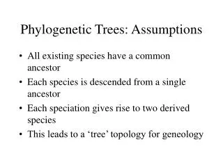
2. Given a set of organisms: • Can we measure similarities, and cluster the organisms into subsets? • Can we form hierarchical clusterings (that is, clusters of clusters of clusters …) that correspond to an evolutionary tree? • Can we calibrate rates of divergence, and thereby date branching events during life history?

3. Note that • We can observe similarities among organisms, or species, both among extant organisms; and, with greater difficulty, extinct ones • It is rare that we can observe evolutionary relationships directly. Generally evolutionary relationship (homology) is an inference from similarities that we can observe • Some dating can be calibrated from geology. However, much dating depends on models and assumptions, and is therefore questionable

4. What is a cluster? • Given a set of objects (species, people, literary texts, protein structures, minerals …) • A cluster is a subset of these objects such that the similarity among the objects in the subset is generally higher than the similarity among the objects in the full set • Clustering depends on property chosen to measure similarity • For instance, focussing on wings would cluster bats with birds; not separate mammals and birds

5. Linnaeus’ SystemaNaturae • Linnaeus (1707-1778) developed a taxonomic system for species • Based on clustering together species with similarities • Main clusters called Kingdoms • Animal, vegetable, mineral • Within each main cluster are subclusters • Hierarchical clustering: clusters of clusters of clusters …

6. http://www.mun.ca/biology/scarr/139416_Natural_classification.jpghttp://www.mun.ca/biology/scarr/139416_Natural_classification.jpg

7. Linnaean hierarchy • Kingdom • Class • Order • Genus • Species • Linnaeus introduced binomial nomenclature: genus/species: For example Homo sapiens, Bostaurus • Higher levels are implied; that is: humans and cows are mammals

8. Linnaean hierarchy • Kingdom • Class • Order • Genus • Species • Linnaeus introduced binomial nomenclature: genus/species: For example Homo sapiens, Bostaurus • Higher levels implied; that is humans and cows are mammals Titian: Rape of Europa

9. Taxonomy now has more levels of clustering • Kingdom • Phylum • Class • Order • Family • Genus • Species There are many intermediate levels also: superfamily, subfamily Below species: variety, strain

10. Objective and subjective aspects of clustering • We have already mentioned the problem of which characters to choose on which to base measurements of similarity. • Even if people agree on the degrees of similarity among element of a set of objects, they may disagree on how finely to cluster them • People are called “lumpers” or “splitters” • To a music major, all chemistry courses one cluster • To a chemistry major: important distinction between physical, analytical, inorganic, organic, biochemical

11. Linnaeus and evolution • When Linnaeus created his taxonomy, it was based solely on his perceived similarities among species • It turned out that the hierarchy largely reflects evolutionary relationships • All the creatures within the same genus or family should be more closely related to each other than they are to creatures in different genuses or families. • Usually true, although Linnaean hierarchy does not always correspond to modern taxonomy

12. Linnaeus v. Huxley • Linnaeus divided the animal kingdom into six classes: mammals, birds, amphibia (including reptiles), fishes, insects and worms.  • Linnaeus therefore considered crocodiles more closely related to salamanders than to birds. • Thomas Huxley, in the 19th century, grouped reptiles and birds together. This is now believed to be correct . • There are, however, much more serious problems in the relation between taxonomy and evolution

13. Similarities are not relationships • Forming hierarchical clusters on the basis of similarities do not necessarily imply biological relationships • Choice of characters with which to measure similarities often ambiguous • Classical methods: palaeontology, comparative anatomy, embryology, in hands of experts, did extremely well • Molecular methods (especially DNA and protein sequences) perhaps more reliable

14. Early attempts to use molecular properties in taxonomy • Especially important for prokaryotes, where standard properties such as skeletal anatomy not possible • Nature of biochemicals – chemotaxonomy • Immunological cross-reactivity • Electrophoretic ‘fingerprinting’ – spread proteome out on a gel • Hybridization of DNAs

15. Genotype and phenotype • Evolutionary relationships fundamentally based on genotype • Palaeontology, comparative anatomy, embryology attempt to reason from phenotype to genotype • So sequence-based methods more direct • However, sequences don’t always give unambiguous answer

16. The species as the ‘atom’ of taxonomy • Taxonomy has been fundamentally the classification of species. • Remember that before Darwin, it was believed that species were immutable • We are still interested in evolutionary trees of species • But it has become clear that it is more difficult to define the concept of species

17. Difficulty in defining species • At base of hierarchy is idea of species. • It is species that Linnaeus and subsequent taxonomists are trying to cluster. • Note: subspecies, varieties, strains … • Difficult to define species • Mutual fertility within group, and infertility outside group, is a major conceptual ingredient • But even for mammals this doesn’t quite work: there are mutually fertile species (tigers, lions) that do not mate in the wild A “tiglon”

18. Whole concept of hierarchy in question • Horizontal gene transfer: incorporation of genetic material from another organism that is not a parent • Example: plasmid exchange among bacteria to distribute antibiotic resistance • Known mechanisms: • Transformation (Avery, McLeod and McCarty, 1944: proof DNA genetic material) • Transduction: virus carries DNA from one organism to another (bacteria, human retroviruses) • Bacterial conjugation: DNA transfer by cell-cell contact

19. From: “Studies on the Chemical Nature of the Substance Inducing Transformation of Pneumococcal Types: Induction of Transformation by a Desoxyribonucleic Acid Fraction Isolated from Pneumococcus Type III.”  J. Exp. Med., 79: 137-158. January 1944. Bacterial conjugation. (Image by C; C. Brinton, Jr., http://biosciences-people.bham.ac.uk/About/staff_profiles_research.asp?ID=205) Bacteriophage infecting E. coli http://www.washington.edu/alumni/partnerships/biology/200710/kerr.html

20. Bacterial transformation http://slic2.wsu.edu Bacterial conjugation knowledgerush.com Bacteriophage infecting cell biology.about.com

21. Horizontal gene transfer makes nonsense of the “tree of life” Picture by W.F. Doolittle

22. To summarize • We want to construct a “tree of life” stating the genealogy of all organisms (or at least all species) • Classical methods based on phenotype not bad • Molecular data – especially DNA sequences – are based directly on genotype • Work as well as anything could • Still problems with horizontal gene transfer • These problems are worse in prokaryotes, worst in earliest life forms (see Doolittle’s picture).22

23. Remaining general problems • Once you choose measures of similarity you can derive a hierarchy • Still left with how you define clusters (lumper-splitter problem) • Whether this represents evolutionary relationships is a question – in view of HGT • Differential rates of change can complicate picture • Can we calibrate molecular similarities to date events in life history?

24. How do we represent hierarchies • Idea of graph: nodes and edges • A tree is a special kind of graph, in which there is only one path from any node to any other node This graph is a tree This graph is not a tree

25. http://www.genealogyintime.com/NewsStories/2009/April/inbreeding_of_spanish_royalty_page2.htmlhttp://www.genealogyintime.com/NewsStories/2009/April/inbreeding_of_spanish_royalty_page2.html Family `tree’ NOT a tree!

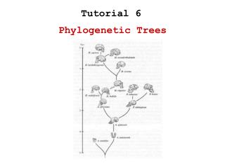
26. How to turn a set of pairwise similarities into a tree • UPGMA method (UnweightedPair Group Method with Arithmetic Mean) • Start by taking each item as a separate subset • Take most closely related pair, form a new node that is their parent • The original pair becomes a two-element subset associated with the higher node • Then take next most closely-related pair of subsets • Similarity/difference between two subsets is the average of the similarities/differences between all pairs of elements from the subsets

27. Number of sequence differences between cytochromes c Data from W.M. Fitch & E. Margoliash, Science 155, 279-284 (1967)

28. UPGMA tree from cytochrome c sequences First two steps: BF closest, join themThen AD next closest, join them http://www.nmsr.org/upgma.htm

29. UPGMA tree from cytochrome c sequences, subsequent steps http://www.nmsr.org/upgma.htm

30. UPGMA method is suitable for deriving hierarchy from any set of objects given a measure of similarity • Problems arise when trying to infer evolutionary relationships, and dating divergences • Consider items sold in different sections of a department store: • Reasonable that men’s and women’s shoes have a common ancestor • Not reasonable that shoes and furniture have a common ancestor

31. Can we trust UPGMA tree as reflecting evolution? • If choice of different similarity measures gives inconsistent results, then there is a problem • Typical similarity measures for molecular biology are sequence similarities, either nucleic acid or protein • Many different measures suggested, basic idea is that the more substitutions in optimal alignment, the more distant the sequences • Quantitatively, correct for back mutation in highly diverged sequences

32. UPGMA assumes constant divergence rates • Suppose there are species that are indeed closely related, but suppose that the cytochrome c of one of them is changing much faster than the other • Then that pair will appear very dissimilar and be separated in the phylogenetic tree • This is an error if we wish to assume that the similarities in the cytochromes c indicate the closeness of the evolutionary relationships

33. Defenses against non-uniform rates of change • Sometimes unusually large rate of change the result of selective pressure • Choose third-base changes as non selective? • Detection of non-uniform rates of change: choose ‘outgroup’ • For instance, if we are dealing with sequences from primates, choose another mammal: cow • Similarity of cow sequence to all primate sequences should be approximately equal • If not, some primate species is changing faster than others

34. Unrooted and rooted trees A rooted tree contains one more bit of information: what node in the graph corresponds tao the last common ancestor Inclusion of an outgroup can allow ‘rooting’ of the tree

35. Cladistic methods • Explicitly assume evolutionary relationship and evolutionary model • Deal specifically with sequences • Start from multiple sequence alignment • Two classical methods: • Maximum parsimony • Maximum likelihood

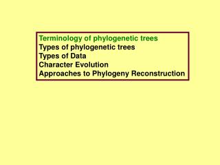
36. Maximum parsimony • Find tree that postulates fewest mutations • Given sequences: ATGC, ATGG, TCCA, TTCA (These appear on bottom line of trees) ● Tree on left postulates four mutations ● Tree on right postulates eight mutations (T→A at position 1 occurs twice) ● Ancestral sequence at each node shown

37. How could you test a method for determining a phylogenetic tree? • Use real data: sequence samples of virus taken from same patient at different times • Use simulated data: set up a model of sequence change, write computer program to implement it, producing a known tree with known final generation of sequences – see whether methods correctly reproduce the tree

38. Time calibration of phylogenetic trees: the ‘Molecular Clock’ • ‘Molecular clock’ hypothesis (Pauling & Zuckerkandl, 1962): suggested that the rate of evolutionary change in the amino acid sequence of each protein family was approximately constant over time, independent of lineage • E. Margoliash (1963): ‘It appears that the number of residue differences between cytochrome C of any two species is mostly conditioned by the time elapsed since the lines of evolution leading to these two species originally diverged.’

39. Problems with molecular clock (F. Ayala) • Different generation times – should the ‘clock’ run at a constant rate per year or per generation? • Population size – genetic drift stronger in small populations, more of evolution is neutral in small populations • General species-specific differences • Functional change in protein studied – stick to non-coding (=??? non-functional??) DNA or silent mutations • Differential selective pressure

40. Calibration of molecular clock • Use dates of species divergence available from classical palaeontology • Dating by geological methods • If there are enough calibration points, then can interpolate • Some well known exceptions to constant rate of sequence divergence have arisen • For instance, the clock runs about 5 times as fast in rodents as in humans (generation time?)

41. Bayes’ theorem: P(A|B) = P(B|A) P(A) / P(B) • The theorem is telling us how to calculate P(A|B) = the conditional probability of A, given the observation B, on which A may depend. • For example: if A = rain and B can = cloudy or sunny, then • P(rain|cloudy) is the probability that it will rain on a cloudy day • P(rain|sunny) is the probability that it will rain on a sunny day (small but not zero) • P(rain|cloudy) is likely to be greater than P(rain|sunny) • P(A) = the prior probability of A. (Without checking the sky today, what is the probability that it will rain = the number of rainy days per year/365) • P(B) = the prior probability of B (number of cloudy days per year/365 or number of sunny days per year /365) • P(B|A) = the conditional probability of B, given A. In our example, P(cloudy|rain) = the probability that it is cloudy, if we know it is raining

42. P(A|B) = P(B|A) P(A) / P(B) • Suppose that in State College there are 66 rainy days per year and 299 (= 365 – 66) dry days • There are 100 cloudy days per year and 265 clear days • 95% of rainy days are cloudy; 5% of rainy days clear • We want to guess whether it will rain today • If we don’t look at the sky we can only estimate: 66/365 = 18% chance of rain • If we observe that it is cloudy, probability of rain is: P(rain|cloudy) = P(cloudy|rain)×P(rain)/P(cloudy) = 0.95 × 0.18 / (100/365) = 62.4% chance of rain

43. P(A|B) = P(B|A) P(A) / P(B) • If we don’t look at the sky we can only estimate: 66/365 = 18% chance of rain • If we observe that it is cloudy, probability of rain is: P(rain|cloudy) = P(cloudy|rain)×P(rain)/P(cloudy) = 0.95 × 0.18 / (100/365) = 62.4% chance of rain • Observation of a contingent quantity (cloudy sky) allows us to correct our a priori probability, 18%, to 62.4%

44. What if we don’t know the numbers? • In the simple example, we had a completely parameterized model and tried to predict an outcome • Alternatively we don’t have the statistics – they are ‘unknown parameters’ – and we observe the sky and the weather over many consecutive days. These are our data. • For any value of the parameters, we can calculate the probability of observing the data. • Those values of parameters that give the highest probability to the data actually observed are our estimate of their values

45. Bayesian inference of phylogenetic trees • Observable: multiple sequence alignment • What phylogenetic tree best accounts for this alignment • Trees depend on model of evolutionary change; a general model being specified by values of parameters such as mutation rate • For any model, can compute the probability of different observed sequence alignments • The likelihood of certain parameter values is the computed probability of observing the actual data, if the parameters have those values

46. More detailed description of parameters • Tree topology and branch lengths • nucleotide or amino acid frequencies • Substitution model parameters • transition/transversion ratio • substitution matrix such as BLOSUM62 • Ancestral sequences • We want to use the observed data to determine the parameters

47. Power of Bayesian methods • Allow for more complex models of evolutionary process • Avoid assumption of constancy of molecular clock along different branches • Allow determination of branching times and rates of evolution along different branches • Calculations can be done with a Markov-Chain-Monte-Carlo (MCMC) approach; this is an efficient way of optimising search in parameter space

48. Suggested reading Holder, M. & Lewis, P.O. (2003). Phylogeny estimation: traditional and Bayesian approaches. Nature Reviews Genetics 4, 275--284.