Download
1 / 32
320 likes | 469 Views
ANALYSIS OF PERFORMANCES IN ELECTRIC AUTOMOBILES (II). PROF. EMILIO LARRODÉ University of Zaragoza. ANALYSIS OF PERFORMANCES IN ELECTRIC AUTOMOBILES. 1. TYRES 2. MECHANICAL RESISTANCE 3. POWER 4. TRANSMISSION 5. CHARACTERISTIC CURVES 6. ADHERENCE 7. ENERGETIC DESIGN

E N D
ANALYSIS OF PERFORMANCES IN ELECTRIC AUTOMOBILES (II) PROF. EMILIO LARRODÉ University of Zaragoza
ANALYSIS OF PERFORMANCES IN ELECTRIC AUTOMOBILES 1. TYRES 2. MECHANICAL RESISTANCE 3. POWER 4. TRANSMISSION 5. CHARACTERISTIC CURVES 6. ADHERENCE 7. ENERGETIC DESIGN 8. WORKING CYCLES
6 ADHERENCE (FRICTION)In this chapter we are going to analyze the four most extreme situations in which the vehicle adherence to the road is usually involved. - maximum acceleration - maximum slope - maximum speed for a given radius during turning - roll over verification Preliminary assumptions and notation:- 50% of total vehicle weight over each axe. - vehicle mass : m- vehicle weight : P- approximate position of gravity center : cdg- approximate height of gravity center : hcdg- wheel base: d- distance from front axe to cdg : a- distance from rear axe to cdg : b- adherence coefficient (friction) : ma- rolling coefficient : m
6.1 MAXIMUM ACCELERATIONS STUDY Maximum accelerations and decelerations of the vehicle occurs during starting and braking. 6.1.1 Braking. Maximum force during braking is calculated in friction and dynamic conditions. Fmax = P · ma = m · g · ma (1.50) Fmax = m · gdeceleration max (1.51) Making equal two previous equations we obtain the value of maximum deceleration: g deceleration max = g · ma (1.52) Once max. deceleration is obtained, we can obtain the braking distance for a given initial speed. To calculate braking distance (D) from vi to vf (vf = 0) 1st we calculate braking time (t). In order to calculate the maximum braking distance we assume initial speed is the vehicle maximum speed (vi = vmax). (1.53) (1.54)
6.1.2 Maximum acceleration. To calculate maximum acceleration by friction conditions, we solve the forces system that can be seen in next figure: where : N1 = normal reaction in front axe wheels N2 = normal reaction in rear axe wheels F1 = Traction force in front axe wheels F2 = Traction force in rear axe wheels R1 = Rolling resistance in front axe wheels R2 = Rolling resistance in rear axe wheels
- 4 wheels drive case. By doing summatory of forces in the displacement axe (x) and in the normal axe (y), we obtain the following equations. P = N1 + N2 (1.55) m · g = F1 + F2 - R1 - R2 (1.56) Moreover, it is verified that : F1 = N1 · ma (1.57) F2 = N2 · ma (1.58) R1 = N1 · m (1.59) R2 = N2 · m (1.60) We obtain the following equation: (N1 + N2) · ma - (N1 + N2) · m = m · g (1.61) substituting in the vehicle weight equation, we have: P · ma - P · m = m · g (1.62) m · g · ma - m · g · m = m · g (1.63) g = g · (ma - m) (1.64)
- Front wheels drive. In this case: (1.65) (1.66) Fmax = N1 · ma (1.67) where m has been calculated by the S.A.E. formula. Time needed to reach determined speed by the vehicle (v) : (1.68) However, this time is not real because that acceleration can not be maintained during all time, but only at the beginning at v = 0 Km/h. If the calculated acceleration here is higher than the maximum acceleration capability obtained during performances analysis, our calculated vehicle will not skip. The maximum acceleration force will be then: Fmax = m · g (1.69)
6.2 MAXIMUM SLOPE In this case we do not consider the aerodynamic resistance. Then, we solve the following system of forces in the next figure: We calculate the total resistance of the vehicle as well as the total traction force as: RT = R1 + R2 + P · sin a (1.70) FT = F1 + F2 (1.71) As we are calculating maximum slope and speed will be very slow, we assume a very low value of acceleration (F = m · g (with m · g = 0 for maximum slope)), that is to say, we assume we are in total traction, then; RT = FT.
Solving the previous system equation F1 + F2 = R1 + R2 + P · sin a (1.72) As : F1 + F2 = P · ma (1.73) R1 + R2 = P cosa · m (1.74) Then : P · ma = P cosa · m + P · sina (1.75) ma = m cosa + sina (1.76) Taking into account: and substituting in the previous equation, we obtain : cos4a [(1 - m2)2 + 4 m2] + cos2a [2(1 - m2) (ma2 - 1) - 4 m2] + (ma2 - 1)2 = 0 (1.77) Solving this equation , obtaining ma depending on the type of soil and m from the SAE formula, we obtain the value of a. Then, the maximum value of the slope expressed in % will be: nmax = 100 · sina (1.78)
6. 3 MAXIMUM VELOCITY IN TURNING To calculate maximum velocity in turning we compose centrifugal force with total resistance and then make equal to adherence or friction force. We assume that slope is 0%. Using following figure: (1.79) where : Fc = centrifugal force RT = total resistance Fad = adherence or friction force
Taking into account that : RT = Rr + Ra + Rp (1.80) Rr = P · m = (1.81) Ra = (1.82) Rp = 0 (for this case) (1.83) Fad = P · ma (1.84) where : r = curve radius (m) v = speed in m/s Because is 4 driving wheels, is independent which axe is. Substituting values: (1.85) Where we can obtain speed v. Taking m as a constant, simplifies the equation.
6.4 ROLL OVER WHILE TURNING To evaluate the possibility of roll over while turning we will solve the forces system which appears in turning. Looking to the figure: where : q= vehicle inclination angle Ld = front way Lt = rear way Fd = force done by the frontal suspension system. Ft = force done by the rear suspension system.
Moreover we define : td = front way / 2 = Ld / 2 (1.86) tt = rear way / 2 = Lt / 2 (1.87) Taking moments respect point O we obtain: Ft · tt + Fd · td + Ft · tt + Fd · td = Fc · hcdg (1.88) 2 · Ft · tt + 2 · Fd · td = Fc · hcdg (1.89) Ft y Fd represent forces done by the suspension system of each frontal and rear suspensions, which are proportional to the displacements of suspension system, and then we can put as : Ft = tt · q · kt (1.90) Fd = td · q · kd (1.91) where : kt = rear suspension stiffness kd = frontal suspension stiffness Establishing the roll over condition (a pair of wheels do not touch the floor): Ft · tt + Fd · td = Fc · hcdg (1.92) and substituting we obtain: tt2 · q · kt + td2 · q · kd = m · v2/r · hcdg (1.93)
Then, we can obtain the vehicle inclination angle q : (1.94) Establishing the forces equilibrium: Fd + Ft = P = m · g (1.95) q · [tt · kt + td · kd] = m · g (1.96) Then : (1.97) and substituting in the equation obtained for the angle q, we allow us to obtain the velocity at which roll over take place. (1.98)
7 ENERGETIC DESIGN Assuming we have a vehicle with the following dimensions, and principal characteristics are: Weight: P (Kg) Speed: v (m/s) Frontal surface: S (m2) Aerodynamic coefficient: Cx Slope: n (%) Rolling coefficient: m Transmission efficiency: hT 1. First, we calculate total resistance to movement (RT), which is the addition of rolling resistance (Rr), aerodynamic resistance (Ra) and resistance to overcome slopes (Rp). RT = Rr + Ra + Rp (1.99) Rr = m · P (1.100) Ra = 1/16 · Cx · S · v2 (1.101) Rp = P · n / 100 (1.102)
2. Once total resistance is obtained, we can calculate the power needed for a given speed v: (1.103) 3. In order to determine the electric power that we need from the electric motor (Pb), it is necessary to check that our electric motor is able to give us the needed power to move the vehicle. This consumed power is calculated applying the efficiency of the electric motor (hE). = f(P) (1.104) 4. Once we know the power of our electric motor, it is possible to determine the energy given by the batteries (Ebt), taking into account the quantity of time that this power is used. Ebt = Pb · t = f(P,t) (1.105)
5. Range of the vehicle (A) at a given speed can be calculated as a function of time that we use the power of the electric motor (t) as: (1.106) Then the equation of the energy given by the battery system can be expressed as: = f(P,A) (1.107) 6. Analyzing the working of the battery system, we need to consider other efficiencies that are related to the charge (hc) and discharge (hd) process. If we add those efficiencies to the calculation of the given energy by the battery system, we will obtain, the total energy that our battery must to have (Ebt0): = f(P,A) (1.108)
7. Once we know the value of the needed energy to impulse the vehicle, we can calculate the weight of our battery (Pbt), knowing the the value of the battery energy capacity (density) (dE), which value will depend on the type of battery used. = f(P,A) (1.109) 8. If we consider the possibility to have a deep discharge of the battery (because a high extension of range), we need to make an over dimensioning of the capacity of the battery by using an efficiency ratio (hdp) which used to be between 80% and 90% of the total capacity needed. Then we have: = f(P,A) (1.110) 9. Now, we can define the specific range concept, (Ae), which give us the vehicle range only as a function of the vehicle weight. Is defined as number of Km driven per battery kilogram, and can be expressed as: = f(P) (1.111)
10. To evaluate the vehicle range (A), and considering the vehicle weight without batteries we can raw the following curves: * Specific range (Km/Kg) * Specific range (Km/Kg) vs. Vehicle weight (Kg) vs. Battery weight (Kg)
* Range (Km) * Range (Km) vs. Battery weight (Kg) vs. Total vehicle weight (Kg)
8 WORKING CYCLES For comparison purposes, we need study how our vehicle behave in different conditions, that is the reason because several kind of working cycles have been defined. These cycles represents the pattern for comparison. So, we have urban cycles, where we include accelerations, braking, and more frequent stops, as well as a more irregular velocity, against the road cycles, where we include a more regular way of driving, and with a less number of accelerations and braking. Working cycles give us medium conditions of driving in urban and suburban circuits.
8.1 CICLE SAE J-227 Is composed by the following periods: 1º acceleration, 2º cruise speed, 3º deceleration, 4º braking, 5º stop. The figure shows different cycle periods where speed is given in Km/h and time in seconds. Time (s)
Values for cycle SAE J-227. A B C D ± ± ± ± v 16 1.5 32 1.5 48 1.5 72 1.5 ± ± ± ± t 4 1 19 1 18 2 28 2 a ± ± ± t 0 19 1 20 1 50 2 cr ± ± ± ± t 2 1 4 1 8 1 10 1 co ± ± ± ± t 3 1 5 1 9 1 9 1 b ± ± ± ± t 30 2 25 2 25 2 25 2 i ± ± ± ± T 39 2 72 2 80 2 122 2
8.2 CYCLE ECE - 15 It is composed by the following periods, urban period which is repeated 4 times and a suburban period. Cycle length is 1180 seconds, 195 s per urban period and 400 s per suburban period.
Example 3. For a given vehicle with the following characteristics: 650 Kg weight, 1350 mm height, and 1481 mm width, aerodynamic coefficient of 0.38, rolling coefficient 0.018 and range in urban cycle 30 Km (transmission and electric motor efficiency are 85 and 87 % respectively). Analyze the total weight of the batteries if the cycle used is the following and we assume that there are no regeneration braking system and the energy capacity of batteries is 30 wh/Kg. Acceleration: from 0 to 47 Km/h 16 s Cruise speed: 47 Km/h 16 s Braking: from 47 to 0 Km/h 7 s Stop: 0 Km/h 25 s cycle time 64 s cycle length 400 m
P = 650 Kg ; hT = 85 % ; m = 0.018 ; hE = 87 % ; Cx = 0.38 ; A = 30 Km S = 0.8 · a · b = 0.8 · 1.35 · 1.481 = 1.6 m2 (1.112) Because it is a urban cycle, we need to know how many times we can repeat the cycle for the given range, taking into account that every cycle has a length of 400 meters: (1.113) * Calculation of total resistance. RT = Rr + Ra + Rp (1.114) (assume that Rp = 0) RT = P · m + 1/16 · Cx · S · v2 = (1.115) = 650 · 0.018 + 0.0625 · 0.38 · 1.6 · (13.05)2 = = 11.7 + 6.47 = 18.17 Kg Range 30.000 = = = # of cycles 75 Length driven in one cycle 400
* Calculation of the power at a speed of 47 Km/h. (1.116) * Calculation of energies for the complete cycle. Eacceleration = Pb · taverage = 3147.15 · 16/2 = 25177.2 ws (1.117) Ecruise = Pb · t = 3147.15 · 16 = 50354.4 ws (1.118) Ecycle = Eacceleration + Ecruise + Ebraking + Estop = (1.119) = 25177.2 + 50354.4 + 0 + 0 = 75531.6 ws ETotal = 75 · Ecycle = 75 · 75531.6 = 5664870 ws (1.120) ETotal = 1573.575 wh (1.121)
* Calculation of battery weight. Energy capability of the battery for a 5 hours discharge: dE = 30 wh/Kg (1.122) Discharge time of the battery in the total cycle: t discharge = t cycle · # cycles = 64 · 75 = 4800 s = 80 min = 1h 20’ (1.123) For this battery, the discharge capability in 1h 20’ corresponds to 70% of the discharge capability in 5 hours. (1.124) To prevent a deep discharge of the battery, an over dimensioning is necessary. In this case we will take: hdp = 90%. = 74.93 / 0.9 = 83.25 Kg (1.125) The calculation of the battery capacity is done taking into account the motor working voltage. Assuming a voltage of V = 24 Volts, the needed capacity will be : CAh = ETotal / V = 1573.575 wh / 24 v = 65.56 Ah (1.126)
Example 4. The vehicle of the previous example is subjected now to a road cycle, where after to get the cruise velocity (60 Km/h), maintain this speed during 90 Km. Calculate the battery weight, assuming that there no exist a regenerative braking system and the energy capability of the battery is 30 wh/Kg. Acceleration: 0 a 30 Km/h 6.4 s Pw = 27.2 Kw (triangle) Acceleration: 30 a 60 Km/h 6 s Pw = 27.2 Kw (rectangular) Cruise speed:60 Km/h tcr s Cycle time: (12.4 + tcr) s Cycle length: 90.000 m
P = 650 Kg ; hT = 85 % ; m = 0.018 ; hE = 87 % ; Cx = 0.38 ; A = 90 Km S = 0.8 · a · b = 0.8 · 1.35 · 1.481 = 1.6 m2 (1.127) There are not repetitive cycles, but we need to calculate the time used at constant speed (cruise speed). A = v · tcr tcr = A / v = 90/60 = 1.5 hours (1.128) * Calculation of total resistance. RT = Rr + Ra + Rp (1.129) (we assume Rp = 0) RT = P · m + 1/16 · Cx · S · v2 = (1.130) = 650 · 0.018 + 0.0625 · 0.38 · 1.6 · (16.66)2 = = 11.7 + 10.54 = 22.24 Kg
* Calculation of motor power at a speed of 60 Km/h. (1.131) * Calculation of the energy of the total cycle. Eacceleration from 0 to 30 Km/h = ½ · Pw · t1 = 0.5 · 27200 · 6.4 = 87040 ws (1.132) Eacceleration from 30 to 60 Km/h = Pw · (t2 - t1) = 27200 · (12.4 - 6.4) = = 163200 ws (1.133) Eacceleration from 0 to 60 Km/h = 87040 + 163200 = 250240 ws (1.134) Due to the necessity to consider the electric motor efficiency: Eacceleration = Eacceleration from 0 to 60 Km/h / hE = 250240/0.87 = = 287632.1 ws = 79.89 wh (1.135) Ecruise = Pb · tcr = 4910.2 · 1.5 = 7365.3 wh (1.136) ETotal = Ecycle = Eacceleration + Ecruise = 79.89 + 7365.3 = 7445.19 wh (1.137)
* Calculation of battery weight. Energy capability of the battery for a 5 hours of discharge: dE = 30 wh/Kg (1.138) Time needed to discharge battery for the given cycle: tdischarge = 1h 30’ (1.139) For this battery, the discharge capability in 1h 30’ corresponds to a 78% of the discharge capability in 5 hours. (1.140) To prevent a deep discharge of the battery, we apply an over dimensioning factor of hdp = 90%. = 318.17 / 0.9 = 353.52 Kg (1.141) The calculation of the battery capacity is done taking into account the working voltage of the motor. If we assume that our motor works at a voltage of V = 24 Volts, the battery capacity will be. C(Ah) = ETotal / V = 7445.19 wh / 24 v = 310.21 Ah (1.142)