Copy Propagation
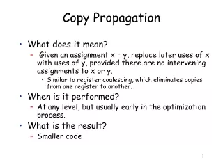
Copy Propagation. What does it mean? Given an assignment x = y, replace later uses of x with uses of y, provided there are no intervening assignments to x or y. Similar to register coalescing, which eliminates copies from one register to another. When is it performed?


Copy Propagation
E N D
Presentation Transcript
Copy Propagation • What does it mean? • Given an assignment x = y, replace later uses of x with uses of y, provided there are no intervening assignments to x or y. • Similar to register coalescing, which eliminates copies from one register to another. • When is it performed? • At any level, but usually early in the optimization process. • What is the result? • Smaller code
Copy Propagation • Local copy propagation • Performed within basic blocks • Algorithm sketch: • traverse BB from top to bottom • maintain table of copies encountered so far • modify applicable instructions as you go
Copy Propagation for instr = i1to in if instr is of the form 'res = opd1 op opd2' flag = replace(opd1, instr) || replace(opd2, instr); /* no short-circuit */ if instr is of the form 'res = var' flag = replace(var, instr); /* replaces var with var2 */ if flag is true /* then we need to update the table */ if instr is of the form 'res = opd1 op opd2' if the table contains any pairs involving res, remove them if instr is of the form 'res = var' insert {(res, var2)} in the table endfor • Algorithm sketch for a basic block containing instructions i1, i2, ..., in replace(opd, instr) if you find (opd, x) in table /* use hashing for faster access */ replace the use of opd in instr with x return true return false
Copy Propagation b = a c = b + 1 d = b b = d + c b = d Example: Local copy propagation on basic block: step instruction updated instruction table contents 1 b = a b = a {(b,a)} 2 c = b + 1 c = a + 1 {(b,a)} 3 d = b d = a {(b,a), (d,a)} 4 b = d + c b = a + c {(d,a)} 5 b = d b = a {(d,a), (b,a)} Note: if there was a definition of 'a' between 3 and 4, then we would have to remove(b,a) and (d,a) from the table. As a result, we wouldn't be able to perform local copy propagation at instructions 4 and 5. However, this will be taken care of when we perform global copy propagation.
Copy Propagation • Global copy propagation • Performed on flow graph. • Given copy statement x=y and use w=x, we can replace w=x with w=y only if the following conditions are met: • x=y must be the only definition of x reaching w=x • This can be determined through ud-chains • there may be no definitions of y on any path from x=y to w=x. • Use iterative data flow analysis to solve this. • Even, better, use iterative data flow analysis to solve both problems at the same time.
Copy Propagation • Data flow analysis to determine which instructions are candidates for global copy propagation • forward direction • gen[Bi] = {(x,y,i,p) | p is the position of x=y in block Bi and neither x nor yis assigned a value after p} • kill[Bi] = {(x,y,j,p) | x=y, located at position p in block BjBi, is killed due to a definition of x or y in Bi } • in[B]=out[P] where P is a predecessor • Initialize in[B1]=, in[B]=U for BB1
Copy Propagation entry entry dead code? c = a + b d = c e = d * d c = a + b d = c e = c * c f = a + c g = e a = g + d a < c f = a + c g = e a = e + c a < c f = d - g f > a f = c - e f > a h = g + 1 h = e + 1 b = g * a h < f b = e * a h < f exit exit
Copy Propagation • Copy propagation will not detect the opportunity to replace x with y in the last block below: • Copy propagation may generate code that does not need to be evaluated any longer. • This will be handled by optimizations that perform redundancy elimination. z >0 Mini quiz: which optimization can handle this? Answer: If we perform an optimization similar to code hoisting (i.e. one that would move the copy either up or down the graph) then copy propagation will be able to update "w=y+z" x = y x = y w = x + z
Constant Propagation • What does it mean? • Given an assignment x = c, where c is a constant, replace later uses of x with uses of c, provided there are no intervening assignments to x. • Similar to copy propagation • Extra feature: It can analyze constant-value conditionals to determine whether a branch should be executed or not. • When is it performed? • Early in the optimization process. • What is the result? • Smaller code • Fewer registers
Redundancy Elimination • Several optimizations deal with locating and appropriately eliminating redundant calculations. • These optimizations require data flow analysis • They include • common subexpression elimination • loop-invariant code motion • partial-redundancy elimination • code hoisting
Common Subexpression Elimination • Local common subexpression elimination • Performed within basic blocks • Algorithm sketch: • traverse BB from top to bottom • maintain table of expressions evaluated so far • if any operand of the expression is redefined, remove it from the table • modify applicable instructions as you go • generate temporary variable, store the expression in it and use the variable next time the expression is encountered. t = a + b x = t ... y = t x = a + b ... y = a + b
Common Subexpression Elimination t1 = a + b c = t1 t2 = m * n d = t2 t3 = b + d e = t3 f = t1 g = -b h = t1 /* commutative */ a = j + a k = t2 j = t3 a = -b if t2 go to L c = a + b d = m * n e = b + d f = a + b g = - b h = b + a a = j + a k = m * n j = b + d a = - b if m * n go to L the table contains quintuples: (pos, opd1, opr, opd2, tmp)
Common Subexpression Elimination • Global common subexpression elimination • Performed on flow graph • Requires available expression information • In addition to finding what expressions are available at the endpoints of basic blocks, we need to know where each of those expressions was most recently evaluated (which block and which position within that block).
Common Subexpression Elimination • Global common subexpression elimination • Algorithm sketch: For each block B and each statement x=y+z, s.t. {y+z}in[B] • Find the evaluation of y+z that reaches B, say w=x+y • Create temporary variable t • Replace [w=y+z] with [t=y+z; w=t] • Replace [x=y+z] with [x=t] • Notes: • This method will miss the fact that b and d have the same value: a = x+y c = x+y b = a*z d = c*z Mini quiz: which optimization can handle this? Answer: Value Numbering
Common Subexpression Elimination entry entry t1 = a + b c = t1 d = a * c t2 = d * d e = t2 c = a + b d = a * c e = d * d f = t1 c = c * 2 c > d f = a + b c = c * 2 c > d g = a * c g = t2 g = a * c g = d * d g > 10 g > 10 exit exit
Loop-Invariant Code Motion • What does it mean? • Computations that are performed in a loop and have the same value at every iteration are moved outside the loop. • Before we go on: What is a loop? • A set of basic blocks with • a single entry point called the header, which dominates all the other blocks in the set and • at least one way to iterate (i.e. go back to the header) • Block Bi dominates block Bj if every path from the flow graph entry to Bj goes through Bi • A loop can be identified by finding an flow graph edge BjBi (called a back edge) s.t. Bi dominates Bj and then finding all blocks that can reach Bj without going through Bi
entry (Loops) B1 The dominator tree shows the dominator relation: each node in the tree is the immediate dominator of its children. Example: B7 is dominated by B1, B3, and B4, but its immediate (closest) dominator is B4 Note: B5 does not dominate B7 because we can go from the entry to B7 through the B6 path. B2 B3 B4 B1 B5 B6 B2 B3 B4 B7 B5 B6 B7 B8 B8 B9 B10 B9 B10 exit
entry (Loops) B1 back edge: B9B1 loop: {B9, B8, B7, B10, B6, B5, B4, B3, B2, B1} B2 B3 back edge: B10B7 loop: {B10, B8, B7} B4 back edge: B8B3 loop: {B8, B7, B10, B6, B5, B4, B3 } B5 B6 back edge: B7B4 loop: {B7, B10, B6, B5, B8, B4} B7 B8 back edge: B4B3 loop: {B4, B7, B10, B8, B6, B5, B3} B9 B10 exit
Loop-Invariant Code Motion • How do we identify loop-invariant computations? • Easy: use ud-chains • But also: • If an computation i depends on a loop-invariant computation j, then i is also loop-invariant. • This gives rise to an inductive definition of loop-invariant computations • An instruction is loop-invariant if, for each operand: 1. The operand is constant, OR 2. All definitions of that operand that reach the instruction are outside the loop, OR 3. There is exactly one in-loop definition of the operand that reaches the instruction, and that definition is loop invariant
Loop-Invariant Code Motion • Algorithm sketch: • Find all loop-invariant instructions • For each instruction i: x=y+z found in step 1, check • that its block dominates all exits of the loop • that x is not defined anywhere else in the loop • that all uses of x in the loop can be reached only by i (i.e. its block dominates all uses of x) • Move each instruction i that satisfies the requirements in step 2 to a newly created pre-header of the loop, making certain that any operands (such as y, z) have already had their definitions moved to the pre-header. • Note: • When applying loop-invariant code motion to nested loops, work from the innermost loop outwards.
Loop-Invariant Code Motion entry Mini quiz: What happens if you perform constant propagation followed by constant folding after the loop-invariant code motion in this loop? b = 2 i = 1 a = b+1 c = 2 i mod 2 = 0 d = a + d e = 1 + d d = -c f = 1 + a i = i+1 a < 2 F T exit
Loop-Invariant Code Motion entry entry b = 2 i = 1 a = b+1 c = 2 t1 = a<2 b = 2 i = 1 a = b+1 c = 2 i mod 2 = 0 i mod 2 = 0 d = a + d e = 1 + d d = -c f = 1 + a d = a + d e = 1 + d d = -c f = 1 + a i = i+1 a < 2 i = i+1 t1 F F T T exit exit
entry entry b = 2 i = 1 a = b+1 c = 2 t1 = a<2 b = 2 i = 1 a = 3 c = 2 t1 = false after constant propagation and constant folding i mod 2 = 0 i mod 2 = 0 d = a + d e = 1 + d d = -c f = 1 + a d = a + d e = 1 + d d = -c f = 1 + a i = i+1 t1 i = i+1 t1 F F T exit exit