Download
1 / 34
340 likes | 521 Views
Unsupervised Optimal Fuzzy Clustering. I.Gath and A. B. Geva. IEEE Transactions on Pattern Analysis and Machine Intelligence , 1989 , 11 (7), 773-781. Presented by Asya Nikitina. Fuzzy Sets and Membership Functions.

E N D
Unsupervised Optimal Fuzzy Clustering I.Gath and A. B. Geva.IEEE Transactions on Pattern Analysis and Machine Intelligence, 1989, 11(7), 773-781 Presented by Asya Nikitina
Fuzzy Sets and Membership Functions • You are approaching a red light and must advise a driving student when to apply the brakes. What would you say: • “Begin braking 74 feet from the crosswalk”? • “Apply the brakes pretty soon”? Everyday language is one example of the ways vagueness is used and propagated. Imprecision in data and information gathered from and about our environment is either statistical (e.g., the outcome of a coin toss is a matter of chance) or nonstatistical (e.g., “apply the brakes pretty soon”). This latter type of uncertainty is called fuzziness.
Fuzzy Sets and Membership Functions We all assimilate and use fuzzy data, vague rules, and imprecise information. Accordingly, computational models of real systems should also be able to recognize, represent, manipulate, interpret, and use both fuzzy and statistical uncertainties. Statistical models deal with random events and outcomes; fuzzy models attempt to capture and quantify nonrandom imprecision.
Fuzzy Sets and Membership Functions Conventional (or crisp) sets contain objects that satisfy precise properties required for membership. For example, the set of numbers H from 6 to 8 is crisp: H = {r∈ ℛ | 6 ≤r ≤ 8} mH= 1; 6 ≤r ≤ 8; mH= 0; otherwise (mH is a membership function) Crisp sets correspond to 2-valued logic: • is or isn’t • on or off • black or white • 1 or 0
Fuzzy Sets and Membership Functions Fuzzy sets contain objects that satisfy imprecise properties to varying degrees, for example, the “set” of numbers F that are “close to 7.” In the case of fuzzy sets, the membership function, mF(r), maps numbers into the entire unit interval [0,1]. The valuemF(r) is called the grade of membership of r in F. Fuzzy sets correspond to continuously-valued logic: • all shades of gray between black (= 1) and white (= 0)
Fuzzy Sets and Membership Functions Because the property “close to 7” is fuzzy, there is not a unique membership function for F. Rather, it is left to the modeler to decide, based on the potential application and properties desired for F, what mF(r) should be like. The membership function is the basic idea in fuzzy set theory; its values measure degrees to which objects satisfy imprecisely defined properties. Fuzzy memberships represent similarities of objects to imprecisely defined properties. Membership values determine how much fuzziness a fuzzy set contains.
Fuzziness and Probability L= {allliquids} ℒ = fuzzy subset of L: ℒ = {all potable liquids} mℒ(A) = 0.91 Pr (B ∈ ℒ) = 0.91
Clustering • Clustering is a mathematical tool that attempts to discover structures or certain patterns in a data set, where the objects inside each cluster show a certain degree of similarity.
Hard clustering assign each feature vector to one and only one of the clusters with a degree of membership equal to one and well defined boundaries between clusters.
Fuzzy clustering allows each feature vector to belong to more than one cluster with different membership degrees (between 0 and 1) and vague or fuzzy boundaries between clusters.
Difficulties with Fuzzy Clustering • The optimal number of clusters K to be created has to be determined (the number of clusters cannot always be defined a priori and a good cluster validity criterion has to be found). • The character and location of cluster prototypes (centers) is not necessarily known a priori, and initial guesses have to be made.
Difficulties with Fuzzy Clustering • The data characterized by large variabilities in cluster shape, cluster density, and the number of points (feature vectors) in different clusters have to be handled.
Objectives and Challenges • Create an algorithm for fuzzy clustering that partitions the data set into an optimal number of clusters. • This algorithm should account for variability in cluster shapes, cluster densities, and the number of data points in each of the subsets. • Cluster prototypes would be generated through a process of unsupervised learning.
The Fuzzy k-Means Algorithm N – the number of feature vectors K – the number of clusters (partitions) q – weighting exponent (fuzzifier; q > 1) uik– the ith membership function on the kth vector ( uik: X [0,1] ) Σkuik= 1; 0 < Σiuik< n Vi– the cluster prototype (the mean of all feature vectors in cluster i or the center of cluster i) Jq(U,V) – the objective function
The Fuzzy k-Means Algorithm Partition a set of feature vectors X into K clusters (subgroups) represented as fuzzy sets F1, F2, …, FK by minimizing the objective function Jq(U,V) Jq(U,V) =ΣiΣk(uik)qd2(Xj – Vi); K N Larger membership values indicate higher confidence in the assignment of the pattern to the cluster.
Description of Fuzzy Partitioning Choose primary cluster prototypes Vi for the values of the memberships Compute the degree of membership of all feature vectors in all clusters: uij=[1/d2(Xj – Vi)]1/(q-1) / Σk [1/d2(Xj – Vi)]1/(q-1)(1) under the constraint: Σiuik= 1
Description of Fuzzy Partitioning Compute new cluster prototypes Vi Vi=Σj[(uij)q Xj] / Σj(uij)q(2) Iterate back and force between (1) and (2) until the memberships or cluster centers for successive iteration differ by more than some prescribed value (a termination criterion)
The Fuzzy k-Means Algorithm • Computation of the degree of membership uij depends on the definition of the distance measure, d2(Xj – Vi): • d2(Xj – Vi) = (Xj – Vi) T-1(Xj – Vi) • = I => The distance is Euclidian, the shape of the clusters assumed to be hyperspherical • is arbitrary=> The shape of the clusters assumed to be of arbitrary shape
The Fuzzy k-Means Algorithm For the hyperellipsoidal clusters, an “exponential” distance measure, d2e(Xj – Vi), based on ML estimation was defined: d2e(Xj – Vi) = [det(Fi)]1/2/Pi exp[(Xj – Vi) T Fi-1(Xj – Vi)/2] Fi– the fuzzy covariance matrix of the ith cluster Pi – the a priori probability of selecting ith cluster h(i/Xj) = (1/d2e(Xj – Vi))/ Σk (1/d2e(Xj – Vk)) h(i/Xj) – the posterior probability (the probability of selecting ith cluster given jth vector)
The Fuzzy k-Means Algorithm It’s easy to see that for q = 2, h(i/Xj) = uij Thus, substituting uij with h(i/Xj) results in the fuzzy modification of the ML estimation (FMLE). Addition calculations for the FMLE:
The Major Advantage of FMLE • Obtaining good partition results starting from “good” classification prototypes. • The first layer of the algorithm, unsupervised tracking of initial centroids, is based on the fuzzy K-means algorithm. • The next phase, the optimal fuzzy partition, is being carried out with the FMLE algorithm.
Unsupervised Tracking of Cluster Prototypes • Different choices of classification prototypes may lead to different partitions. • Given a partition into k cluster prototypes, place the next (k +1)th cluster center in a region where data points have low degree of membership in the existing k clusters.
Unsupervised Tracking of Cluster Prototypes Compute average and standard deviation of the whole data set. Choose the first initial cluster prototype at the average location of all feature vectors. Choose an additional classification prototype equally distant from all data points. Calculate a new partition of the data set according to steps 1) and 2) of the fuzzy k-means algorithm. If k, the number of clusters, is less than a given maximum, go to step 3, otherwise stop.
Common Fuzzy Cluster Validity Each data point has K memberships; so, it is desirable to summarize the information by a single number, which indicates how well the data point (Xk) is classified by clustering. • Σi(uik)2partition coefficient • Σi(uik)loguikclassification entropy • maxiuikproportional coefficient The cluster validity is just the average of any of those functions over the entire data set.
Proposed Performance Measures “Good” clusters are actually not very fuzzy. The criteria for the definition of “optimal partition” of the data into subgroups were based on the following requirements: Clear separation between the resulting clusters Minimal volume of the clusters Maximal number of data points concentrated in the vicinity of the cluster centroid
Proposed Performance Measures Fuzzy hypervolume, FHV, is defined by: Where Fi is given by:
Proposed Performance Measures Average partition density, DPA, is calculated from: Where Si, the “ sum of the central members”, is given by:
Proposed Performance Measures The partition density, PD, is calculated from:
Sample Runs In order to test the performance of the algorithm, N artificial m-dimensional feature vectors from a multivariate normal distribution having different parameters and densities were generated. Situations of large variability of cluster shapes, densities, and number of data points in each cluster were simulated.
FCM Clustering with Varying Density The higher density cluster attracts all other cluster prototypes so that the prototype of the right cluster is slightly drawn away from the original cluster center and the prototype of the left cluster migrates completely into the dense cluster.
(a) (b) • Fig. 3. Partition of 12 clusters generated from five-dimensional multivariate Gaussian distribution with unequally variable features, variable densities and variable number of data points ineach cluster (only three of the features are displayed). • Data points before partitioning • (b) Partition of 12 subgroups using the UFP-ONC algorithm. All data points gave been classified correctly.
Conclusions • The new algorithm, UFP-ONC (unsupervised fuzzy partition-optimal number of classes), that combines the most favorable features of both the fuzzy K-means algorithm and the FMLE, together with unsupervised tracking of classification prototypes, were created. • The algorithm performs extremely well in situations of large variability of cluster shapes, densities, and number of data points in each cluster .