Download
1 / 32
320 likes | 342 Views
As the number of assets in the portfolio increases, note how the number of covariance terms in the expansion increases as the square of the number of variance terms. As we add additional assets, we can lower overall risk.

E N D
As the number of assets in the portfolio increases, note how the number of covariance terms in the expansion increases as the square of the number of variance terms
As we add additional assets, we can lower overall risk. Lowest achievable risk is termed “systematic”, “non-diversifiable” or “market” risk Standard deviation Lowest risk with n assets Diversifiable / idiosyncratic risk Systematic risk 1 2 ... 40 20 No. of shares in portfolio
Percentage of risk on an individual security that can be eliminated by holding a random portfolio of stocks US 73 UK 65 FR 67 DE 56 IT 60 BE 80 CH 56 NE 76 International 89 Source: Elton et al. Modern Portfolio Theory
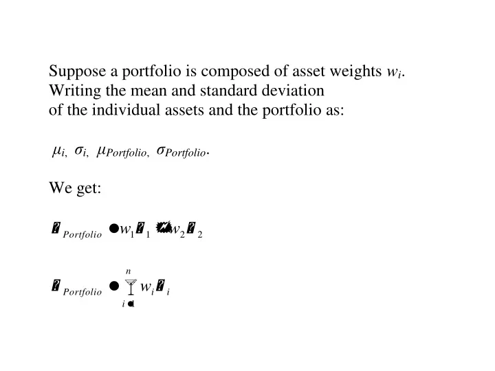
Add assets…especially with low correlations • Even without low correlations, you lower variance as long as not perfectly correlated • Low, zero, or (best) negative correlations help lower variance best • An individual asset’s total variance doesn’t much affect the risk of a well-diversified portfolio
Building the efficient frontier: combining two assets in different proportions Mean return 0, 1 0.5, 0.5 0.75, 0.25 1, 0 Standard deviation
Risk and return reduced through diversification Mean return r = - 1 r = +0.5 r = +1 r = - 0.5 r = 0 Standard deviation
Efficient frontier of risky assets μp A x x x x x x x B x x x x x x x x x C sp
Capital Market Line and market portfolio (M) Capital Market Line =Tangent from risk-free rate to efficient frontier μ B M μm A μm - rf rf a s sm
Individual preferences Mean return I2 > I1 μp I2 I1 B A ERp Z s Y sp Standarddeviation
Capital Market Line and market portfolio (M) μ B Investor A reaches most preferred M-V combination by holding some of the risk-free asset and the rest in the market portfolio M giving position A IA M μm A μm - r r a s sm
Capital Market Line and market portfolio (M) IB μ B B is less risk averse than A. Chooses a point that requires borrowing some money and investing everything in the market portfolio M μm A μm - r r a s sm
Some lessons from our toy exercise for daily returns • It’s laborious to compute the efficient set • Curvature is not that great except for negatively correlated assets • We “know” that these means and covariances are going to be bad estimates of next weeks process…so how stable do we think asset returns are generally…. …is it just a question of longer samples or do covariances etc change over time?
Issues in using covariance matrix for portfolio decisions • Expected returns are very volatile – past not a good guide • Covariances also volatile, but less so • If we try to estimate covariances from past data • (i) we need a lot of them (almost n2/2 for n assets) • (ii) lots of noise in the estimation • But a simplifying model seems to fit well:
What is β? Could get it from past historic patterns (though experience shows these are not stable and tend to revert to mean… …adjustments possible (Blume, Vasicek) Could project it from asset characteristics (e.g. if no market history) Dividend payout rate, asset growth, leverage, liquidity, size (total assets), earnings variability
Why use single index model? (Instead of projecting full matrix of covariances) • Less information requirements • It fits better!