Download
1 / 46
480 likes | 585 Views
Evaluation of Wax Deposition and Its Control During Production of Alaska North Slope Oils. Annual Report Jan – Dec, 2006 University of Alaska Fairbanks Kansas University ConocoPhilips 22 January 2007. Project Objectives.

E N D
Evaluation of Wax Deposition and Its Control During Production of Alaska North Slope Oils Annual Report Jan – Dec, 2006 University of Alaska Fairbanks Kansas University ConocoPhilips 22 January 2007
Project Objectives • Evaluate the mechanisms and environments leading to wax deposition during ANS oil production • Develop predictive models and give guidance for potential wax-free production • Evaluate methods and techniques to prevent and control wax deposition during production
Wax Deposition Diagram Initial Reservoir Condition ● Liquid P-T Path Critical ● Point Pressure Liquid + Gas Wax Envelope Gas Temperature
To Achieve Wax-Free Production • P-T path for production must stay outside of the wax envelope • Requires in-depth understanding of • Thermodynamic properties of crude oil • Heat transfer characteristics of production string and the influence of permafrost • Wax deposition under dynamic conditions
Work Done • Density determination of all tank oil samples as function of temperature • Molecular weight determination of crude oil using Cryette A for all 28 tank oil samples • Determination of tank oil WATs by cross polar microscope (CPM) (12 samples) and viscometer (28 samples) • Composition analysis of crude oil using GC-MS • Selection of suitable thermodynamic model for wax precipitation • Bubble point curve prediction program
Work Done (Cont.) • Development of program for plus fraction splitting into suitable number of components • Algorithm development for prediction of WAT of the oil • Development of analytical solution for wellbore geometry (by KU) • Development of numerical solution for wellbore geometry (by KU) • Development of computer program for solid-liquid flash problem (by KU)
Density Measurement • Density measured using ANTON-PAAR density-meter • Density as a function of temperature is determined for modeling purpose
Density Measurement Results (Cont.) Sample density at 15 0C
Density Measurement Results (Cont.) Density of all samples as a function of temperature
Molecular Weight Measurement • Need for measurement of molecular weight • Used for calculating critical properties of fractions which are required for modeling • Instrument- Cryette A • Measures depletion in freezing point and relates it to the concentration of solvent (benzene) and hence to the molecular weight of the solute • Kf = 5.120C/mole, ΔFP= Meter Reading
Wax Appearance Temperature (WAT) measurement • Dead oil WAT measurement using Brookfield Programmable viscometer, Model LVDV-II+ • Sudden increase in viscosity is used as indication of sign of wax appearance • Dead oil WAT measurement using Cross Polar Microscope (CPM) • Polar light makes the wax crystals shine as soon as they appear
WAT measurement by Viscometry Programmable LVDV-II+ Viscometer Data gathering PC Heating/Refrigerating bath Brookfield viscometer
CCD Hot Stage Top View Analyzer 10 50 20 Cooling Gas Hot Stage 360° Rotatable stage Polarizer IR - Filter WAT By CPM(for dead oil)
WAT by Viscometry Spindle: SC4-21 RPM: 200 Temp range: 50 to 0oC WAT = 20.3oC WAT plot of sample 06
Composition Analysis • Need for composition analysis • Used for identifying the type of crude • Required for modeling phase equilibrium and properties of hydrocarbon mixtures • Method of analysis • GC-MS • Flame Ionization Detector
Plus Fraction Splitting • Need for plus fraction splitting • Not well defined composition gives gross information and make EOS models behave poorly • Extended composition distribution gives better results • Pedersen’s method used for splitting plus fraction into suitable number of components • Program flexible to consider splitting upto desired carbon number depending on the requirement
Plus Fraction Splitting Results North Sea Crude Oil sample
Work Done at University of Kansas (KU) • Thermodynamic Model • Heat-Transfer Model • Dynamic Wax Deposition Model
Heat-Transfer Model Objective: • Establish temperature profiles in production string. Approach: • Model heat exchanges between producing fluids, production string, insulation materials and formation rock/permafrost using total system energy balance. • Generate system temperature profiles by solving total-system- energy-balance equation numerically using finite-difference method.
Total System Energy Balance • Heat loss into the formation = Total heat flow from center of well to cement/formation interface • Newton’s Law of Cooling: Where A: crossectional-area T: temperature Ut: overall heat-transfer coefficient Equating Eqs. (1) and (2) yields
Overall Energy Balance of Heat Transfer Into Formation Rock Assumptions: • Physical properties of system components independent of temperature. • Steady-state heat flow in the formation rock. • Radial heat flow from wellbore into formation rock. • Heat transfer from center of wellbore to cement/formation interface (0 → rh) represented by an overall heat transfer coefficient, Ut.
Overall Energy Balance of Heat Transfer Into Formation Rock Boundary Conditions:
Numerical Model Finite Difference Approximation:
Simulation of Heat Loss from Cement/Formation Interface into Formation Rock Steam Injection Example Well Depth= 5,000 ft, Ke = 1.0 Btu/hr-ft-°F, ce = 0.21 Btu/lb-°F, cf = 1.0 Btu/lb-°F, Tf = 600 °F, Te = 80 °F, Ut = 3.4274 Btu/hr-sq ft-°F, ρ = 167 lb/ft3, rto= 0.146 ft, rh = 0.5 ft.
Analytical Solutions • Analytical solutions of heat conduction in an infinite circular cylinder bounded by a surface can be used to calculate cement/formation temperature change vs. time (Willhite, 1967). where f(t):transient heat conduction function solved analytically
Validation of Numerical Model with Analytical Solutions Eq. (3) can be rearranged as Eq. (4) can be used to calculate f(t) using temperature data from numerical model. • Numerical model can be validated by comparing f(t)analytical vs. f(t)numerical
Analytical vs. Numerical Solutions Steam Injection Example Well During first 200 hours of steam injection, cement/formation interface temperatures calculated using Numerical model match analytical solutions well.
Thermodynamic Model Phase Composition in Solid-Liquid Equilibrium(Experimental data from Dauphin et al. 1999) Predictions from our thermodynamic model match experimental data well.
Future Work • Measure WAT of remaining tank oil and live oil samples by CPM • Complete GC-MS characterization • Conduct PVT Analysis • Complete GC-FID analysis • Develop program to predict WAT • Development of the thermodynamic model to predict cloud point
Acknowledgement We gratefully acknowledge the financial support from AEDTL/NETL/DOE