Download
1 / 22
310 likes | 591 Views
Lecture 4: Fitting distributions: goodness of fit. Goodness of fit Testing goodness of fit Testing normality An important note on testing normality!. 30. 20. Frequency. 10. Expected. 0. 20. 30. 40. 50. 60. Observed. Fork length. Goodness of fit.

E N D
Lecture 4: Fitting distributions: goodness of fit • Goodness of fit • Testing goodness of fit • Testing normality • An important note on testing normality! Bio 4118 Applied Biostatistics
30 20 Frequency 10 Expected 0 20 30 40 50 60 Observed Fork length Goodness of fit • measures the extent to which some empirical distribution “fits” the distribution expected under the null hypothesis Bio 4118 Applied Biostatistics
Accept H0 Reject H0 Goodness of fit: the underlying principle 30 Expected Observed 20 • If the match between observed and expected is poorer than would be expected on the basis of measurement precision, then we should reject the null hypothesis. 0 Frequency 30 20 10 0 20 30 40 50 60 Fork length Bio 4118 Applied Biostatistics
Expected Observed Frequency Category/class Testing goodness of fit : the Chi-square statistic (C2) • Used for frequency data, i.e. the number of observations/results in each of n categories compared to the number expected under the null hypothesis. Bio 4118 Applied Biostatistics
0.3 c2 = 8.5, p = 0.31 accept Probability 0.2 p = a = 0.05 0 c2 (df = 5) 0 5 10 15 20 How to translate C2 into p? • Compare to the 2 distribution with n - 1 degrees of freedom. • If p is less than the desired level, reject the null hypothesis. Bio 4118 Applied Biostatistics
Expected Observed Frequency Category/class Testing goodness of fit: the log likelihood-ratio Chi-square statistic (G) • Similar to C2, andusually gives similar results. • In some cases, G is more conservative (i.e. will give higher p values). Bio 4118 Applied Biostatistics
0.3 Probability 0.2 0 c2/C2/G (df = 5) 0 5 10 15 20 c2 versus the distribution of C2 or G • For both C2 and G, p values are calculated assuming a 2 distribution... • ...but as n decreases, both deviate more and more from2. C2/G, very small n C2/G, small n c2 Bio 4118 Applied Biostatistics
Assumptions (C2 and G) • n is larger than 30. • Expected frequencies are all larger than 5. • Test is quite robust except when there are only 2 categories (df = 1). • For 2 categories, both X2 and G overestimate 2, leading to rejection of null hypothesis with probability greater than , i.e. the test is liberal. Bio 4118 Applied Biostatistics
What if n is too small, there are only 2 categories, etc.? • Collect more data, thereby increasing n. • If n > 2, combine categories. • Use a correction factor. • Use another test. More data Classes combined Bio 4118 Applied Biostatistics
Corrections for 2 categories • For 2 categories, both X2 and G overestimate 2, leading to rejection of null hypothesis with probability greater than i.e. test is liberal. • Continuity correction: add 0.5 to observed frequencies. • Williams’ correction: divide test statistic (G or C2) by: Bio 4118 Applied Biostatistics
The binomial test • Used when there are 2 categories. • No assumptions • Calculate exact probability of obtaining N - k individuals in category 1 and k individuals in category 2, with k = 0, 1, 2,... N. Probability 0 1 2 3 4 5 6 7 8 9 10 Number of observations Binominal distribution, p = 0.5, N = 10 Bio 4118 Applied Biostatistics
An example: sex ratio of beavers • H0: sex-ratio is 1:1, so p = 0.5 = q • p(0 males, females) = .00195 • p(1 male/female, 9 male/female) = .0195 • p(9 or more individuals of same sex) = .0215, or 2.15%. • therefore, reject H0 Bio 4118 Applied Biostatistics
Multinomial test • Simple extension of binomial test for more than 2 categories • Must specify 2 probabilities, p and q, for null hypothesis, p + q + r = 1.0. • No assumptions... • ...but so tedious that in practice C2 is used. Bio 4118 Applied Biostatistics
Multinomial test: segregation ratios • Hypothesis: both parents Aa, therefore segregation ratio is 1 AA: 2 Aa: 1 aa. • So under H0, p =.25, q = .50, r = .25 • For N = 60, p < .001 • Therefore, reject H0. Bio 4118 Applied Biostatistics
Expected under hypothesis of normal distribution Observed Frequency Category/class Goodness of fit: testing normality • Since normality is an assumption of all parametric statistical tests, testing for normality is often required. • Tests for normality include C2 or G, Kolmogorov-Smirnov, Wilks-Shapiro & Lilliefors. Bio 4118 Applied Biostatistics
1.0 Cumulative normal density function 0.8 Normal probability density function 0.6 50.00% F 0.4 2.28% 0.2 68.27% 0 -3s -2s -s m s 2s 3s Cumulative distributions • Areas under the normal probability density function and the cumulative normal distribution function Bio 4118 Applied Biostatistics
Frequency Category/class C2 or G test for normality Expected under hypothesis of normal distribution • Put data in classes (histogram) and compute expected frequencies based on discrete normal distribution. • Calculate C2. • Requires large samples (kmin = 10) and is not powerful because of loss of information. Observed Bio 4118 Applied Biostatistics
NEDs Normal Non-normal X “Non-statistical” assessments of normality • Do normal probability plot of normal equivalent deviates (NEDs) versus X. • If line appears more or less straight, then data are approximately normally distributed. Bio 4118 Applied Biostatistics
1.0 0.8 0.6 Cumulative frequency 0.4 Dmax 0.2 X Komolgorov-Smirnov goodness of fit • Compares observed cumulative distribution to expected cumulative distribution under the null hypothesis. • p is based on Dmax, absolute difference,between observed and expected cumulative relative frequencies. Bio 4118 Applied Biostatistics
1.0 0.8 Dmax 0.6 Cumulative frequency 0.4 0.2 4.0 4.5 5.0 5.5 6.0 Wing length An example: wing length in flies • 10 flies with wing lengths: 4, 4.5, 4.9, 5.0, 5.1, 5.3, 5.5, 5.6, 5.7, 5.8, 5.9, 6.0 • cumulative relative frequencies: .1, .2, .3, .4, .5, .6, .7, .8, .9, 1.0 Bio 4118 Applied Biostatistics
Lilliefors test • KS test is conservative for tests in which the expected distribution is based on sample statistics. • Liliiefors corrects for this to produce a more reliable test. • Should be used when null hypothesis is intrinsic versus extrinsic. Bio 4118 Applied Biostatistics
An important note on testing normality! • When N is small, most tests have low power. • Hence, very large deviations are required in order to reject the null. • When N is large, power is high. • Hence, very small deviations from normality will be sufficient to reject the null. • So, exercise common sense! Bio 4118 Applied Biostatistics