Download
1 / 89
890 likes | 919 Views
Explore lossy compression reducing geometry size, balancing quality and compression ratio. Learn key steps like mesh conversion, quantization, and encoding for improved storage and bandwidth efficiency.

E N D
Geometry Compression Michael Deering, Sun Microsystems SIGGRAPH (1995) Presented by: Michael Chung
Geometry CompressionWhat is it? • Lossy technique for reducing the size of geometry representation.
Motivation • Save bandwidth and transmission time in graphics accelerators and networks. • Save storage space in main memory and on disk.
Proposed Contributions • Technique for lossy compression ratios of between 6 and 10 to 1 • Claims only slight losses in object quality • Depends on original representation format and final quality level desired
Geometry CompressionWhat is it? • Trade-off between quality (subjective) and amount of compression. • Compression steps can be reversed for decompression
Geometry CompressionWhat is it? • Goal: represent geometry with geometry compression instructions
Insights • Reduce size of geometry representation in several ways. • Reuse vertices in triangle strip via reference • Bit shaving • Geometry is local, encode deltas • Normals as indices
Compression Steps • Convert triangle data to generalized triangle mesh • Quantization of positions, colors, normals • Delta encoding of quantized values • Huffman tag-based variable-length encoding of deltas • Output binary output stream with Huffman table initializations and geometry compression instructions
Compression Steps • Convert triangle data to generalized triangle mesh • Quantization of positions, colors, normals • Delta encoding of quantized values • Huffman tag-based variable-length encoding of deltas • Output binary output stream with Huffman table initializations and geometry compression instructions
Step 1: Conversion to Generalized Triangle Mesh generalized triangle strip generalized triangle mesh • Generalized triangle strip • Specifies vertices with four vertex replacement codes (2 bits): • Replace oldest • Replace middle • Restart clockwise • Restart counterclockwise
Step 1: Conversion to Generalized Triangle Mesh • Generalized triangle strip (example)
Step 1: Conversion to Generalized Triangle Mesh • Generalized triangle strip (example)
Step 1: Conversion to Generalized Triangle Mesh • Generalized triangle strip (example)
Step 1: Conversion to Generalized Triangle Mesh • Generalized triangle strip (example)
Step 1: Conversion to Generalized Triangle Mesh • Generalized triangle strip (example)
Step 1: Conversion to Generalized Triangle Mesh • Generalized triangle strip (example)
Step 1: Conversion to Generalized Triangle Mesh • Generalized triangle strip (example)
Step 1: Conversion to Generalized Triangle Mesh • Generalized triangle strip (example)
Step 1: Conversion to Generalized Triangle Mesh • Generalized triangle strip (example)
Step 1: Conversion to Generalized Triangle Mesh generalized triangle strip generalized triangle mesh • Generalized triangle mesh • Generalized triangle strip • Mesh buffer • 16 slot queue • 4 bit index • Explicitly push vertices onto mesh buffer for reuse. • We save because only 4 bits are required to reference old vertex.
Step 1: Conversion to Generalized Triangle Mesh • Generalized triangle mesh (example)
Step 1: Conversion to Generalized Triangle Mesh • Generalized triangle mesh (example)
Step 1: Conversion to Generalized Triangle Mesh • Generalized triangle mesh (example)
Step 1: Conversion to Generalized Triangle Mesh • Generalized triangle mesh (example)
Step 1: Conversion to Generalized Triangle Mesh • Generalized triangle mesh (example)
Step 1: Conversion to Generalized Triangle Mesh • Generalized triangle mesh (example)
Step 1: Conversion to Generalized Triangle Mesh • Generalized triangle mesh (example)
Step 1: Conversion to Generalized Triangle Mesh • Generalized triangle mesh (example)
Step 1: Conversion to Generalized Triangle Mesh • Generalized triangle mesh (example)
Step 1: Conversion to Generalized Triangle Mesh • Generalized triangle mesh (example)
Step 1: Conversion to Generalized Triangle Mesh • Generalized triangle mesh (example)
Step 1: Conversion to Generalized Triangle Mesh • Generalized triangle mesh (example)
Compression Steps • Convert triangle data to generalized triangle mesh • Quantization of positions, colors, normals • Delta encoding of quantized values • Huffman tag-based variable-length encoding of deltas • Output binary output stream with Huffman table initializations and geometry compression instructions
Step 2: Quantization • Some parts of the geometry may require more or less precision than others.
Step 2: Quantization • Some parts of the geometry may require more or less precision than others. • So, the amount of quantization we perform per position, normal, and color is variable.
Step 2: Quantization • Position • 32-bit floating-point coordinates are wasteful. • 8-bit exponent allows an unnecessary range of values. • 24-bit fixed-point mantissa offers unnecessary precision.
Step 2: Quantization • Position • Based on empirical visual tests, allow at most 16 bits per component (X, Y, Z)
Step 2: Quantization • Color • Linear reflectivity values R, G, B, (optional) A • Range from 0.0 to 1.0 per component • cap state bit sets alpha ON and OFF • At most 12 unsigned fraction bits per component
Step 2: Quantization • Normal • 96 bits can represent up to 296 different normals • We don’t need so many • Angular density of 0.01 radians between normals visually indistinguishable • This is about 100,000 normals distributed over a unit sphere • 48 bits to represent a normal (16 bits per X, Y, Z) • We can do better than 48 bits per normal • Use clever indexing to represent ~100,000 normals with 18 bits…
Step 2: Quantization • Normal • 96 bits can represent up to 296 different normals • We don’t need so many • Angular density of 0.01 radians between normals visually indistinguishable • This is about 100,000 normals distributed over a unit sphere • 48 bits to represent a normal (16 bits per X, Y, Z) • We can do better than 48 bits per normal • Use clever indexing to represent ~100,000 normals with 18 bits…
Step 2: Quantization • Normal • 96 bits can represent up to 296 different normals • We don’t need so many • Angular density of 0.01 radians between normals visually indistinguishable • This is about 100,000 normals distributed over a unit sphere • 48 bits to represent a normal (16 bits per X, Y, Z) • We can do better than 48 bits per normal • Use clever indexing to represent ~100,000 normals with 18 bits…