Download
1 / 87
870 likes | 880 Views
f(t). m. x(t). f d (t). C (Ns/m). k (N/m). LINEAR CONTROL. x(t) is the output variable and is measured by a displacement sensor. The output of a sensor is always an electrical output mainly voltage.

E N D
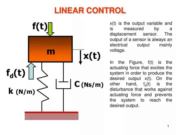
f(t) m x(t) fd(t) C(Ns/m) k(N/m) LINEAR CONTROL x(t) is the output variable and is measured by a displacement sensor. The output of a sensor is always an electrical output mainly voltage. In the Figure, f(t) is the actuating force that excites the system in order to produce the desired output x(t). On the other hand, fd(t) is the disturbance that works against actuating force and prevents the system to reach the desired output.
V1 (Force, Moment, etc.) Gact Actuators: Actuators are used to drive the engineering systems. DC motors, servo motors, hydraulic and pneumatic system elements are the basic type of actuating elements. The inputs of the actuators are also voltage. One can write a transfer function in order to model the behaviour of an actuator. (Voltage)
Sensors: Sensors are the basic components of a control system that are used to measure the output/outputs of the system in order to obtain a feedback signal. The output of a sensor is mainly a voltage signal. One can write a transfer function in order to relate the input and output of the sensor. The input of a sensor is a physical event, temperature, pressure, displacement, velocity, acceleration, magnetic flux, rate of the fluid flow etc.) (Voltage) Displacement,pressure, temperature V2 Gsens
-Fd + V1 F(t) x(t) V2 Gact Gsens + 0.1 Volt/m 100 N/Volt OPEN-LOOP CONTROL
Objective: The desired steady-state value of x(t) is 0.05 m. In this case, the sensor output voltage is calculated as The input voltage which is sufficient to obtain the output voltage, V2 is calculated as m=200 kgc=300 Ns/mk=5000 N/m The steady-state behaviour doesn’t include time variations and the system considered as static, then
V2(t) V2ss=0.005 Volt The Figure shows that, desired x(t) value is achieved if the external disturbance Fd is zero. If Fd is not zero!
Fd=0 V2(t) Fd=80 N Time (second)
-Fd (Error) + V1 Vref E x(t) V2 F(t) + Gact Gcont Gsens + - 0.1 Volt/m 100 N/Volt Feedback Can we obtain desired x(t) even if Fd is not zero. This is the main concern of a control process. This can be achieved via the impementation of a closed-loop control.
The form of the transfer function of the controller is the most important parameter in a control application. Gcont can be Proportional, Derivative, Integralor a suitable combination of these three choices.
Kp is the proportional constont, Ki is the integral constant and Kd is the derivative constant. For proportional control, Gcont=Kp Vref=0.005 Volt, Fd=80 N Let’s take Kp=1000
Desired Open-loop V2(t) Closed-loop, Kp=1000. Time (second)
Closed-loop, Kp=10000 Desired V2(t) Open-loop Closed-loop, Kp=1000 ess Kp Time (second) ess
For proportional-derivative (PD) control, Gcont=Kp+KdsKp=10000, Kd=100
PD Control by Simulink Reference Voltage:0.005 Volt Disturbance:-80 N
Desired V2(t) Time (second) PD Control by Simulink
Gc PID Control by Simulink Controller
PID Control: Kp=1000, KI=1000, Kd=1000 Desired Output PI Control: Kp=1000, KI=1000 PD Control: Kp=1000, Kd=1000 P Control: Kp=1000 Effect of the PID parameters on the output
STABILITY OF LINEAR CONTROL SYSTEMS Among the many forms of performance specifications used in design, the most important requirement is that the system be stable. An unstable system is generally considered to be useless. The stability of a control system is directly related to the location of the roots of the charactersitic equation D(s). s-plane j Stable region Unstable region 0 Stable region Unstable region
V2(s) V1(s) 100 D(s) Example 1: Consider an open-loop control system
-6.7913 -2.2087 V2(t) V2ss=6.66 Time (s) s-plane D(s)=s2+9s+15 by MATLAB s1=-2.2087 s2= -6.7913 >>a=[1 9 15]; >> roots (a) The two roots of D(s) are in the left hand side of the s-plane. It can be easily said that the open-loop system is stable. Response of the system to a unit step input can be obtained by MATLAB as >>ns=[100]; >>ds=[1 9 15], >>step(ns, ds)
D(s) Example 2: V2(s) V1(s) 100 >>a=[1 3 75]; >> roots (a) s1=-1.5+8.53i s2=-1.5-8.53i
Response of the system to a unit step input can be obtained by MATLAB as >>ns=[100]; >>ds=[1 3 75], >>step(ns, ds) s-plane -1.5+8.53 i V2ss=1.33 -1.5-8.53 i
Example 3: V2(s) V1(s) 100 The real part of the roots are zero. No roots on the right-half s-plane and system is said to be marginally stable. s1=+3.8730i s2= -3.8730i >>a=[1 0 15]; >> roots (a) D(s)
Response of the system to a unit step input can be obtained by MATLAB as >>ns=[100]; >>ds=[1 0 15], >>step(ns, ds) s-plane 3.873 i -3.873 i V2(t) Time (s)
D(s) Example 4: V2(s) V1(s) 100 The real part of the roots are positive. Two roots are on the right-half s-plane and system is said to be unstable. s1=1+3.8730i s2=1-3.8730i >>a=[1 -2 16]; >> roots (a)
Response of the system to a unit step input can be obtained by MATLAB as >>ns=[100]; >>ds=[1 -2 16], >>step(ns, ds) s-plane 1+3.873 i 1-3.873 i V2(t) Unstable Time (s)
+ V2(s) R(s) K - Example 4: System Consider a closed-loop control system Controller Mason Formula:
V2(s) + R(s) K -
V2(s) + R(s) K - Forward Path Loop By using Mason formula D(s) Is the closed-loop control system stable? For what values of K, the system is said to be stable?
Routh-Hurwitz criterion: This criterion is an algebraic method that provides information about the stability of a linear time invariant system that has a characteristic equation with constant coefficients. The criterion tests whether any of the roots of characteristic equation lie in the right-half s-plane. The number of roots that lie on the j axis and in the right half plane is also indicated. s3 1 K+9 s2 5 3K+5 s1 0 s03K+5 0 All terms must have the same sign. The number of positive roots is equal to the change in the sign.
K+9 >0 , K>-9 3K+5 > 0, K> -1.66 0.4K+8>0, 0.4K>-8, K>-8/0.4, K>-20 K>-1.66 System is stable for all positive K values. s1= -1.1333 + 3.3941i s2= -1.1333 - 3.3941i s3= -2.7334 For K=10; Response of the system to a unit step input can be obtained by MATLAB as >>ns=[10 30]; >>ds=[1 5 19 35], >>step(ns, ds) s-plane -1.1333+3.3941i -2.7334 -1.1333-3.3941i
Response to a unit step input, V2(t) V2(t) Time (s) Stable
Example 1: + V2(s) R(s) K - D(s)
K>0, 24K>0, 80K>0 K>0 s5 1 50000 24K s4 600 K 80K s3 0 s2 0 s1 s0
K=1x10⁵ K=5x10⁵ K=2.34x10⁵ K=2.1386x10⁷ K=3x10⁷ Unstable Stable Unstable
Example 2: + V2(s) R(s) K - s3 1 200 s2 30 K s1 0 s0 K<6000 0 < K< 6000 K>0 Kcritical=6000
By MATLAB, >>K=2000; >>ns=[K]; >>ds=[1 30 200 K]; >>step(ns,ds) V2(t) K=2000 Time (sec) Stable
By MATLAB, >>K=6000; >>ns=[K]; >>ds=[1 30 200 K]; >>step(ns,ds) Marginally stable K=6000 V2(t) D(s)=s3+30s2+200s+6000 >>ds=[1 30 200 6000]; >>roots(ds) p1=-30.0000 p2= 0.0000 +14.1421i p3=0.0000 -14.1421i Time (sec)