Statistical methods in cosmology André Tilquin (CPPM) tilquin@cppm2p3.fr

1. Statistical methods in cosmologyAndré Tilquin (CPPM) tilquin@cppm.in2p3.fr m, ,w0,w1 2

2. Outlook • General problem • The frequentist statistic • Likelihood, log-likelihood and 2 • Fisher analysis and limitation • The Bayesian statistic • The Bayes theorem • Example and interpretation. • Summary

3. General problem(1) • Let assumes we have N Supernovaeat different redshift • and a given model: • How to find the best curve ? • We look for the closest curve with respect to the data points: • But the worst measured points should have less weight.

4. General problem(2) • The problem now is: • Find the kvalue such that 2is minimum • Computed the errors on kstarting from the errors on mi Statistic is necessary

5. Freqentist statistic Definition: Probability is interpreted as the frequency of the outcome of a repeatable experiment. Central limit theorem If you repeat N times a measurement, and for N, the measurement distribution (pdf) will be a Gaussian distribution around the mean value with a half width equal to the error of your experiment.

6. Maximum likelihood(=0). What is the best curve ? Answer : The most probable curve ! The probability of the theoretical curve is the product of each individual point to be around the curve: We have to maximze L with respect tok  Because it is simpler to work with sum: We have to minimizewith respect tok 

7. Some 2property Probabilityand2 : By definition Definition in matrix form: Second derivative: • The first2derivative gives le minimum • The second2derivative givesthe weight matrix = inverse of the error matrixindependent of the measured data points.

8. Computing errors When the 2is defined on measured variables (i.e magnitude), how to compute the errors on physical parameters, k? We perform a Tailor expansion ofthe2around minimum: =0 If the transformation m(k) is linear, then: The second derivative of the 2is a symetric positive matrix The error on kare Gaussian

9. Computing errors(2) Simple case: Jacobi If m(k, zi) is linear Error on physical parameter are deduced by a simple projection on the kspace parameter(linear approximation) Fisher analysis Independant of the measured points If m(k, zi) is not linear: Fisher is a good approximation if:

10. Exemple: variables change • Assumewe know errors on m et  , (no correlation). We would like to compute errors on S=m+ et D=m-: • We construct the covariance matrix • We construct the Jacobian: • We project: • We inverse V:

11. External constraint or prior • Problem: Using SN we would like to measured ( m,) knowingthat from the CMB we have :T=m+=1.010.02. • This measurement is independent from the SN measurement. So we can add it to 2. All the previous equations are still correctby replacing: And the Jacobi:

12. Minimisation of2 and bias estimate We Tailor expandthe2 around ko: We apply the minimum condition in k We get the first order iterative équation: If theoritical model is linear, this equation is exact (no iteration)

13. Non-linéarity • If m(k) is linearin kthen: • If errors on mi are Gaussianthen errors on kwill be • 2(k) is exactly a quadratic form • The covariance matrix is positive and symetric • Fisher analysis is rigorously exact. • On the contrary only 12is rigorously exact: Fisher matrix is a linear approximation. • The only valid properties are: • Best fit is given by => • The « s » sigma error is given by solving: 12 = 2min +s2

14. 2=min2+1 Fisher analysis Secondary minimum - + asymetric error Non linearity: example Evolution of12- min2 : SNAP simlation, flatness at 1 % Rem:This secondary minimum is highly due to non linearity.

15. Non Gaussianity When errors on observables are not Gaussian, only the minimum iterative equation can be use. So go back to the definition: “Probability is interpreted as the frequency of the outcome of a repeatable experiment” and do simulation: Gedanken experiments • Determine the cosmological model {k0} by looking for the best fit parameters on data. This set of parameters is assumed to be the true cosmology. • Compute the expected observables and randomize them inside the experimental errors, taking into account non Gaussianity. Do the same thing with prior. • For each “virtual” experiment, compute the new minimum to get a new set of cosmological parameters ki • Simulate as many virtual experiments as you can • The distributions of these “best fit” value {ki} give the errors: • The error matrix is given by second order moments: Ui,j={<ij> - <i> <j>} positive define • The error on errors scale as σ(σ) ~σ/√2N

16. Bayesian statisticorThe complexity of interpretation 1702-1761 (paper only published in 1764)

17. Bayesian theorem. measurement Posterior to measurement Prior to measurement Normalization factor=Evidence Normalization factor is the sum over all possible posteriors to ensure unitarily of probability. Where > means after and < means before.

18. Example • Question: Suppose you have been tested positive for a disease; what is the probability that you actually have the disease? -Efficiency of the test: -Disease is rare: What is the Bayesian probability? Why a so small Bayesian probability (16%) compare to Likelihood probability of 95%? Which method is wrong?

19. Intuitive argument. • Over 100 people, the doctor expect 1 people has a disease and 99 have no disease. If doctor makes test to all people: • 1 has a disease and will probably have a positive test • 5 will have a positive test while they have no disease 6 positive tests for only 1 true disease So the probability for a patient to have a disease when the test is positive is 1/6~16% =>Likelihood is wrong? • In the previous argument doctor used the whole population to compute its probability: • 1% disease and 99% not disease before the test • He have assumed that the patient is a random guy. The patient state before the measurement is a superposition of 2 states • /patient> = 0.01*/desease>+0.99*/healthy> • But what about yourself before the test? • /you> = /disease> or /healthy> but not both state in the same time /you>  /patient> =>Bayesian is wrong?

20. Which statistic is correct? Both! • But they do not answer to the same question!: • Frequentist: If “my” test is positive what is the probability for me to have a disease? 95% • Bayesian: If “one of the” patient has a positive test what is the probability for this patient to have a disease? 16% • Different questions give different answers! Conclusion: In Bayesian statistic, the most important is the prior because it can change the question! It’s the reason why statistician like Bayesian statistic, because just playing with prior can solve a lot of different problems. On the contrary, in Scientific works, we should care about prior and interpretation of the Bayesian probability.

21. Summary • Both statistics are used in cosmology and give similar results if no or week priors are used. • The frequentist statistic is very simple to use for gaussian errors and rather linear model. Errors can easily be computed using Fisher analysis. • Bayesian statistic might be the only method to solve very complex problem. But warning about probability interpretation! • For complex problem, only simulation can be used and are lot of computing time. • When using priors in both cases a careful analysis of results should be done

22. References • http://pdg.lbl.gov/2009/reviews/rpp2009-rev-statistics.pdf • http://www.inference.phy.cam.ac.uk/mackay/itila/ • http://ipsur.r-forge.r-project.org/ • http://www.nu.to.infn.it/Statistics/ • http://en.wikipedia.org/wiki/F-distribution • http://www.danielsoper.com/statcalc/calc07.aspx • If you have any question or problem, send me an e-mail: tilquin@cppm.in2p3.fr

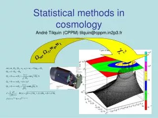
23. Kosmoshow: cosmology in one click Choose different probes Actions: Kosmosfit: fitting and error computing Main table: SN definition Fitting options Click icon and then in any place for help Prior definition. Your cosmology used for simulation Predefines survey: Data or simulation Define different dark energy parameterization Manage files and load predefine survey Parameters to be fitted

24. Server : 166.111.26.237 • Connect to the server: • User: student • Pwd: thcaWorkshop • Create a directory with your name: • mkdirtilquin • source /cosmosoft/environment/idl-env.sh • Go to your work directory • cp /home/tilquin/kosmoshow/*.* . • idl kosmoshowsc Or download from http://marwww.in2p3.fr/~tilquin/

25. Non-linearity: computing errors If m(k) is not linear, errors on k is not gaussian. Fisher analysis is no more correct. If one use it, results should be verify a posteriori. To estimated the errors we should come back to the first definition of the 12and solve the equation 12 = 2min +1 If we want to estimate () what about M ? How to take care of correlation ? How to marginalize over M ? • Average answer (simulation) • Most probable answer (data) It can be shown than both methods are equivalent for simulation if simulated point are not randomized. mmes = mth

26. Bayesian evidence • Bayes forecasts •  method: •  define experiment configuration and models •  simulate data D for all fiducial parameters •  compute evidence (using the data from b) •  plot evidence ratio B01 = E(M0)/E(M1) •  limits: plot contours of iso-evidence ratio •  ln(B01) = 0 (equal probability) •  ln(B01) = -2.5 (1:12 ~ substantial) •  ln(B01) = -5 (1:150 ~ strong) •  Computationally intensive: need to calc. 100s of • evidences

27. 39% 39% Graphical interpretation (contour) • The equation: define an iso-probability ellipse.  -/4 68%

28. Systematic errors Définition:Systematic error isall that is not statistic. Statistic: If we repeat « n » the measurement of the quantity Q with a statistical error Q, the average value <Q> tendsto the true value Q0with an errorQ/n. Systematic:Whatever is the number of experiments, <Q> will never tends to Q0better than the systematic errorS. How to deal with: If systematic effect is measurable, we correct it, by calculating <Q-Q> with the error Q’2= Q2+ Q2 If not, we add the error matrices: V’ = Vstat+Vsyst and we use the general formalism. Challenge:The systematic error should be less than the statistical error. If not, just stop the experiment, because they won !!!!

29. Error on the z parameter SNAP mesure mi et zi with errorsm et z. Redshift is used as a paremeter on the theoritical model and its error is not on the 2. But the error on z leads toan error on m(m,,zi) Thus, the error on the difference mi-mthis: