Download
1 / 26
520 likes | 1.22k Views
CATS 1-D XL. One-Dimensional Tolerance Stackup Spreadsheet. by Ken Chase and Jonathan Wittwer Brigham Young University. Complex Assemblies. 3s. Capability. Process Variation. Mean. Standard Deviation. -1s. +1s. Rejects. LL. UL. -3s. +3s. A frequency plot shows how a

E N D
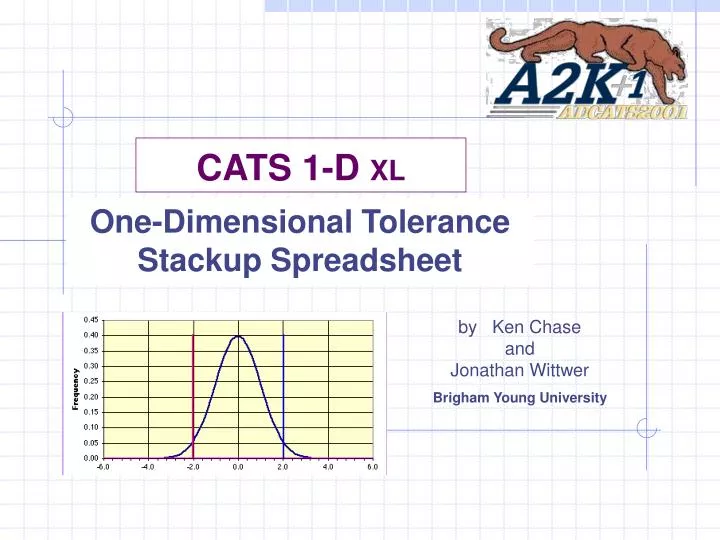
CATS 1-D XL One-Dimensional Tolerance Stackup Spreadsheet by Ken Chase and Jonathan Wittwer Brigham Young University
3s Capability Process Variation Mean Standard Deviation -1s +1s Rejects LL UL -3s +3s A frequency plot shows how a process varies from the mean
Models for Predicting Assembly Tolerance Stackup • Worst Case (WC) • Statistical (RSS) • Six Sigma (6s) • Measured Data (Meas)
Centering the Mean Center Rejects Xmean LL UL Centering the process in the LL/UL window minimizes rejects
3s Capability Decrease Variation Decrease Standard Deviation Reduce rejects LL UL -3s +3s
LL UL -6s -5s -4s -3s -2s -1s 0 +1s +2s +3s +4s +5s +6s ±3s ±4.5s ±6s Higher s Values Mean Higher Quality
Controlling Variation Leads to Higher Yields and Fewer Defects LimitsYield Defects ±3s 99.73% 2700 / Million ±4.5s 99.99966% 3.4 / Million ±6s 99.9999998% 2 / Billion
Controlling Variation Leads to Higher Yields and Fewer Defects LimitsYield Defects ±3s 99.73% 2700 / Million ±4.5s 99.99966% 3.4 / Million ±6s 99.9999998% 2 / Billion
Mean Shifts Happen Mean Shift Mean variation is time-dependent due to tool wear, temperature, etc.
Accounting for Mean Shifts 1.5s 4.5s LL UL The Six Sigma Model allows the engineer to model assembly variation due to mean shifts
Measures of Process Capability UL LL Process Capability Index: 3 ± s Cp adjusted for k: k UL LL Cpk= Cp(1-k) 6 ± s
UL LL 3 ± s k UL LL 6 ± s 6 Variation Defined RSS: 6s: where Cpk= Cp(1-k) and
3s Capability Six SigmaDynamic Mean Shift 99.73% (Short Term) 95.45% (Long Term) LSL USL -3s +3s Comparing Short and Long Term Variation Distribution of parts tool wear Distribution of parts when tool is new. when tool is old. - tolerance + tolerance min. max. Figure 7. Scenario 3. As the tool wears, the mean of the most recent parts shifts from the left to the right
Requirements for High Quality 99.9999998% (Short Term) LL UL 99.99932% (Long Term) -6s +6s 6s Capability A goal of 4.5s long term requires a 6s process in the short term
Excel Statistical Functions NORMDIST(x,mean,stand_dev,T/Fflag) =area under the Normal distrib at point x NORMSDIST(z) =area under the Standard Normal distrib STANDARDIZE(x,mean,stand_dev) =(x - mean)/stand_dev NORMSINV(Probability) =z corresp to a given probability(for z <5) SUMSQ(G1:G25)^0.5 =square root of the sum of squares of si
a Yield (1- a) Rejects Z Yield Fraction a Source 3s 6s 15 Place Math Tables 0.998650101968370000 0.999999999013000000 6th Order Polynomial Fit 0.998650187471804000 0.999999998751939000 Excel 0.998650032776765000 0.999999999009878000 Reject Fraction (1-a) Source 3s 6s 15 Place Math Tables * 0.001349898031629990 0.000000000987000000 6th Order Polynomial Fit 0.001349812528196100 0.000000001248061000 Excel 0.001349967223235000 0.000000000990122000 StatisticalFunction Accuracy * the 6s value is from an alternate source, accurate to 12 places.
Yield and Rejects Calculated in s units, %, or parts-per-million
X = 0 Standard Normal Distribution Transformation ZL ZU Mean Standard Deviation sx = 1.0 Z (s units) Used to determine % rejects from standard tables. Does not show mean shift. Transformed data all looks alike.
Modified Normal Distribution LL UL Shows the mean shifts Shows the quality levels Allows all 3 curves to be plotted for comparison
What can CATS 1-D users expect? Probably won’t see: An end to poverty and misery All men treating each other as brothers World peace But, you might notice: An increased understanding of the role of statistics in design Fewer problems on the factory floor Engineering and production talking to each other without shouting.