Download
1 / 12
130 likes | 370 Views
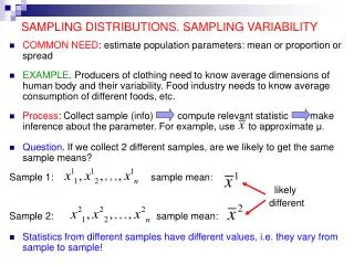
Random Sampling and Sampling Distributions Chapter 6. “He stuck in his thumb, Pulled out a plum and said ‘what a good boy am I!’” old nursery rhyme. Topics and Goals for Chapter 6. Random Sampling Sample Statistics and Relation to Population Parameters

E N D
Random Sampling and Sampling DistributionsChapter 6 “He stuck in his thumb, Pulled out a plum and said ‘what a good boy am I!’” old nursery rhyme MGMT 242
Topics and Goals for Chapter 6 • Random Sampling • Sample Statistics and Relation to Population Parameters • Sampling Distribution for Sample Mean-- ”The Central Limit Theorem” • Checking Normality-The Normal Probability Plot • samples from normal distributions • positively skewed distributions • negatively skewed distributions • distributions with outliers MGMT 242
Populations and Samples • A population is a large collection (theoretically, for the mathematician, infinite) of the individuals or items of interest (e.g. consuming public, machine line production items, etc.) • To measure characteristics of the population we have to take a sample (smaller number). • If we take a random sample, it is equally likely that any member of the population will be included in the sample. MGMT 242
Random Sampling • Sample represents population only if each member of population equally likely to be included in sample. • Types of random sampling (see also Chapter 16): • Simple Random Sampling (SRS)-- sample whole population • Stratified Random Sampling divide population into groups and sample from each group; for example, in polls, divided country into four geographical regions and sample from each • Cluster Sampling Divide population into groups and take a sample of a few groups from the total--e.g., looking at hospital performance, sample patients in few hospitals randomly chosen from all hospitals in the state. MGMT 242
Sample Statistics • Sample Mean: xbar = (1/N) xi , where “xbar” is x with a bar over it; the sum is taken over all values of the random variable X measured in the sample of N units. xbar is an estimator of the population mean, . • Sample Standard Deviation: s = {[1/ (N-1)] (xi- xbar)2 }(1/2 s is an “unbiased estimate” of the population standard deviation, . Note that for large samples (large N), N-1 N MGMT 242
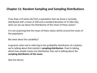
Sampling Distribution for Sample Means:The Central Limit Theorem--1 • In general (which means almost always), no matter what distribution the population follows, the distribution of the sample means follows a normal distribution with • mean µsample means (for the population of sample means) equal to µ, the mean for the parent population, and • standard deviation of the means sample means= /N. This means that the larger the sample size, the more accurately we estimate the mean. MGMT 242
Sampling Distribution for Sample Means:The Central Limit Theorem-2 • The histogram on the left is for a sample from a uniform distribution (0 to 100). The sample mean is 50.2 and the sample standard deviation is 29.3 (100/12) MGMT 242
Sampling Distribution for Sample Means:The Central Limit Theorem-2 • The histogram on the left is for the means of 150 samples, each size 9 (N = 9). The average of these 150 means is 49.4 and the standard deviation of these 150 sample means is 9.8 which is about (100/[129]), the population standard dev-iation of the mean. MGMT 242
Normal Probability Plots (“P-plots”) • The procedure to get this plot, which tests whether data follow a normal distribution procedure, is the following: • 1) order the N data; • 2) assign a rank from 1--the lowest--to N--the highest value; • 3) find the centile score of the mth data point from the relation centile score = m/(N+1)--e.g the 1st data point out of 100 has a fraction approximately 1/101 lower; the 100th data point has a fraction 100/101 lower; • 4) find the z-value (standard normal variate) corresponding to the centile score (this would be the z-score or N-score). • 5) plot the observed points versus the z-score; • If the points fall approximately on a straight line, the distribution is a normal distribution. MGMT 242
Normal Probability Plots (“P-plots”) Examples Exam 2 scores were negatively skewed (range: 49-100, Q1=90, median=92, Q3= 94 rank ordered value z-score Exam 2 1 0.02 -2.10 49 2 0.04 -1.80 72 3 0.05 -1.61 78 4 0.07 -1.47 79 5 0.09 -1.35 81 6 0.11 -1.24 85 7 0.13 -1.15 86 8 0.14 -1.07 87 9 0.16 -0.99 89 etc. …. MGMT 242
Normal Probability Plots (“P-plots”) Examples (cont.) This Pplot for Exam 2 scores is from the “Statplus” addin; note that the axes are inter-changed from the previous (conventional) order: Nscore is y-axis, actual score is x-axis rank ordered value z-score Exam 2 1 0.02 -2.10 49 2 0.04 -1.80 72 3 0.05 -1.61 78 4 0.07 -1.47 79 5 0.09 -1.35 81 etc. …. MGMT 242
Qualitative Appearance of P-plots MGMT 242