Download
1 / 40
400 likes | 512 Views
4. 1. 9. 7. 5. 6. 8. 13. 10. 2. 3. 12. 11. “Real problems”. Nodal patterns on graphs. 1.The Laplace operator on metric graphs ( “ Quantum Graphs ” ) 2.The Laplace operqtor on discrete graphs. “ Quantum graphs ”. “Discrete graphs”. The Schroedinger operator on graphs:

E N D
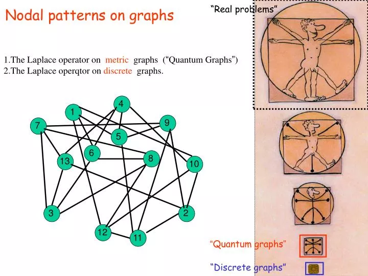
4 1 9 7 5 6 8 13 10 2 3 12 11 “Real problems” Nodal patterns on graphs 1.The Laplace operator on metric graphs (“Quantum Graphs”) 2.The Laplace operqtor on discrete graphs. “Quantum graphs” “Discrete graphs”
The Schroedinger operator on graphs: 1. The wave function 2. The wave equation On each bond: 3. The boundary conditions at the vertices i = 1,…V Neumann : . Dirichlet : The Schroedinger operator is self – adjoint with real and non-negative discrete spectrum
The 1stsurprising numerical evidence (Tsampikos Kottos, U.S., (1997)) = cumulative level-spacing distribution
Proof (idea) : 1. Traceformulae and the length spectrum (Roth, Kottos & US) Schroedinger spectrum: {kn2} 2. Identify all “1 bond” orbits: Q : (Q is constructed as the minimal basis for the length spectrum) A finite search! {Lb}, b=1,B Non commensurability of the bond lengths! 3. Construct all metric stars: Thus, the lengths and the connectivity matrix are uniquely recovered
Conclusion: isospectral but not isometric graphs must have commensurate bond lengths! Example: (Michail Solomyak)
Sunada isospectral quantum graphs Principle: building blocks, transpositions 73 b c Central vertex not an isometry Boundary vertex
Counting nodal domains on graphs But how do we count ? Metric count ( = 8) Schapotschnikow (2006): On tree graph, the nth eigenfunction has n nodal domains Berkolaiko (2007): For a graph of rank r, the number of nodal domains of the n’th eigenfunction is bounded in the interval Discrete count ( = 1)
Resolving isospectrality Isospectral tree graphs – Because of the tree nature of the isospectral graphs, metric count does not resolve isospectrality. Discrete count does resolveisospectrality for some isospectralpairs. Numerical evidence.(Shapira & Smilansky 2005) The length spectrum from the nodal sequence (numerical)
a 2c 2b N D 2b b b D N a a 2a c c 2c N D Constructing isospectral pair using the Dihedral D4 symmetry Rami Band {D. Jakobson, M. Levitin, N. Nadirashvili and I.Pelterovich}, Martin Sieber
Discrete nodal count N D 2b b b D N a a 2a c c 2c N D • Theorem 1 – Let GI and GII the graphs below. Denote with {in} the sequence of discrete nodal count of the graph Gi. Then {In} is different from {IIn} for half of the spectrum. GII GI
Discrete nodal count GI N N N N D D plus minus N D N N N D D D D N D N • Obsevation – The transplantation that takes an eigenfunction of GI with eigenvalue k and transforms it to eigenfunction of GII with eigenvalue k is: GI GII
Discrete nodal count I=1 I=1 I=2 I=2 II=1 II=2 N D N D I=2 I=2 I=1 I=1 II=2 II=1 GI D N GII • Geometrical representation of the transplantation of a certain eigenfunction
Discrete nodal count • Calculate h(x) - the distribution function of
Discrete nodal count • Calculate h(x) - the distribution function of Ergodic principle {In} is different from {IIn} for half of the spectrum.
Metric nodal count N D 2b b b D N a a 2a c c 2c N D • Theorem 2 – Let GI and GII the graphs below. Denote with {in} the sequence of metric nodal count of the graph Gi. Then { In} is different from { IIn} for half of the spectrum. GII GI
Metric nodal count N D N D GI D N GII • Presenting the formula for the number of metric nodal domains (Gnutzmann, Smilansky & Weber) • Number of nodal points on the bond (i,j) is given by ( or if ϕi=0 or ϕj=0 then) • Number of metric nodal domains:
Metric nodal count N D N D GI D N GII • Recall that on tree graph, the nth eigenfunction has n nodal domains (Schapotschnikow 2006). So that: • Nodal count difference is: • Again, we use the ergodic principle to calculate the distribution function h(x) of In- IIn : { In} is different from { IIn} for half of the spectrum.
Discrete Laplacians Graphs: G: Connected, finite, simple graph with V vertices and B bonds Connectivity : Ci,j vi= valency = jCi,j Ci,j 2 {0,1} Discrete Laplacian Li,j = - Ci,j + vii,j Secular equation: ZV() = det (IV – L) = 0 The spectrum is non-negative, 0 in the spectrum Task: Generate random ensembles which have a given connectivity and study - Spectral statistics - Eigenvectors statistics - Conditions for the existence of limit distributions when V !1 Definition : A regular graph G(V,v) is a connected graph with V vertices all having the same valency vi = v.
Numerics: Spectral density: (McKay) Nearest level distribution
Nodal domains: Let =(1, 2, … , V) be an eignevector of the graph Laplacian with eigenvalue . The number of nodal domains () : # of maximally connected subgraphs on which the i have the same sign Courant (1922) : Arrange the eigenvectors by increasing values of the corresponding eigenvalues. Let n be the number of nodal domains of the n’th eigenvector. Then: n n Nodal sequence:1,2, … , V = 3
Interior vertex 2. Morphology of nodal domains
Example: rectangular grid ¸ = v ¸ < v ¸ > v
Eigenvectors correlations G(4000,3) v = 3-regular graph The “tree approximation” is expected to be exact for k <1/2 log V TexPoint fonts used in EMF. Read the TexPoint manual before you delete this box.: AAAAAAAAAAA
Counting nodal domains Courant bound Assuming the tree approximation and Guassian distribution V=3 V=6
3. Nodal domains vs Percolation on random v-regular graphs We consider random regular G(V,v) graphs in the limit
Percolation on Graphs (Erdos and Renyi, Alon et. al., Nachmias and Peres) Start with a random v-regular graph on V vertices. Perform an independent p-bond percolation : Retain a bond with a probability p Delete a bond with a probability 1- p Phase transition at pc = 1/(v-1): Denote by L the number of vertices in the largest connected component pc p < pc p > pc 1/V1/3 E(L) ~o(V2/3) E(L) ~ V2/3 E(L)~o(V2/3) V1/3 Bond percolation ~ Vertex percolation
4 1 9 7 5 6 8 13 10 3 2 12 11 Phase transition in the eigenstates of the discrete Laplacian ? For a given eigenvalue, and we apply the following procedure: We enumerate the vertices according to the decreasing value of the eigenstate at the vertex.1st vertex : Maximum value Vth vertex : Minimum value
Next, we delete vertices which have an index larger than (and all the bonds which are attached to them). We denote this graph by 4 1 5 3 2
Compute the ratio between the cardinality of the largest connected component of the sub-graph and the cardinality of . ( ) 4 1 5 3 2
Critical percolation vs eigenvalue for 3 d-regular graphs. Numerical and Mean field results (Yehonatan Elon)
nodal counting and isospectrality Given an arbitrary function on the vertices (not necessarily and eigenfunction of a Laplacian) How does the connectivity of the graph limit the number of nodal domains? How to count? Idan Oren: Theorem: Denote by max the maximum number of nodal domains on a graph, and by the chromatic number of the graph. Then the following (optimal) bound holds: Optimal bound: for a tree graph = 2 and max = V for a complete graph = V and max= 2
Explicit formulae for counting nodal domains (Idan Oren and Rami band) Given a graph G and a function fi on the vertices. Denote si= Sign [ fi ] (f) = the number of sign flips on a graph = # { ( i, j ) | si sj < 0 }. (1): (f) = ¼ (s,Ls) where L is the graph Laplacian. Proof: (s,Ls) = (si - sj)2 Ci,j A flip contributes 4 to the sum (2): (f) = ¼ (s,Ls) – (r - c) +1; where r = B - V+1 is the number of independent cycles in G (The rank of the fundamental group of G) c = the number of independent cycles in G with the same si Proof: For a tree (f) = (f) +1 and r = c =0. Continue by induction on r. (3): Construct an auxiliary graph with connectivity (f) = the degeneracy of the lowest eigenvalue for the corresponding Laplacian Efficient for simulations (using SVD).
Corollary : Let G and H be an isospectral pair of graphs, G bipartite and H not, Then, the nodal counts for the eigenfunctions with the largest eigenvalue are different, G > H.
Conclusions Nodal domains – counting and morphology A surprising junction of many fields in Math. Phys. Open Problems: For non-separable systems (Graphs incl): How to count nodal domains? Trace formula for nodal domains. Counting nodal intersections. Resolution of isospectral domains Nodal domains in d (>2) dimensions Thank you for your attention