Download
1 / 19
190 likes | 202 Views
Principles: Range edges. What determines the edge of geographic ranges? There are changes in local population dynamics at the edge of a distribution, and more net losses than net gains These population level changes are brought about by:

E N D
Principles: Range edges What determines the edge of geographic ranges? • There are changes in local population dynamics at the edge of a distribution, and more net losses than net gains These population level changes are brought about by: • Changes in abiotic factors (physical barriers, climate factors, absence of essential resources) and biotic factors (impact of competitors, predators or parasites) • Genetic mechanisms that prevent species from becoming more widespread. Abiotic/biotic factors are only limiting because a species has not evolved the morphological / physiological / ecological means to overcome them.
Principles: Response curves • Plot of species presence with variation in some environmental variable. • Most models assume a Gaussian response, but in fact it is seldom Gaussian, and may take on a variety of shapes. Especially in complex communities, response curves may exhibit truncated forms due to biotic interactions. • The ability of the chosen model to represent this response curve is critical to model performance.
Specifics: Niche-based modelling Species Distribution Environmental Variables Model Calibration Yes Independent evaluation dataset No 70/30% Random Calibration/Evaluation Sample Independent evaluation dataset Model Evaluation Final Model used to project current and future distributions
Niche-based modelling –assumptions • Assumptions: • Environmental factors drive species distribution • Species are in equilibrium with their environment • Limiting variables – are they really limiting? • Coincidence with climate or climate shift • Evidence for species dying/not reproducing due to climate • Collinearity of variables • Assumption of assembly rules: niche assembly vs dispersal assembly • Static vs dynamic approaches: data snapshot or time series response?
Cautionary note on modelling in general • Risk of all models: GIGO- Garbage in, garbage out • Need to understand assumptions, explicit and implicit • Models are an abstraction of reality, meant to improve our understanding of core processes.
Variables and their selection • Species only select their habitats in the broadest sense (Heglund 2002), and distribution patterns are the cumulative result of a large number of fine scale decisions made to maximize resource acquisition. • The more accurately these fine-scale resources can be approximated and access quantified, the better the model should perform if all models were equal. • Predictions at broad scales can use broader environmental variables, often associated with the fundamental niche, • Finer scale predictions need to concern themselves more with those variables that determine the realized niche. (Pearson & Dawson 2003)
Environmental Variables • MAP, Psummer, Pwinter • MAT, Tmin, Tmax, Tmin06 • Soil (pH, texture, organic C, fertility) • Avoid indirect measures of a variable which is a challenge • project into the future e.g. slope, aspect, altitude • Difficult variables – Solar radiation, wind
Derived Variables • Growing degree days (e.g. base 5°C) • PET – Thornthwaite, Priestly-Taylor, Linacre • Water Balance – Crudely defined as MAP – PET • Favourable soil moisture days– Modelled using e.g. ACRU, WATBUG • Palmer Drought Stress Index – PDSI Program
BIOCLIM Environmental Variables • Mean Temperature of Warmest Quarter • Mean Temperature of Coldest Quarter • Annual Precipitation • Precipitation of Wettest Month • Precipitation of Driest Month • Precipitation Seasonality • Precipitation of Wettest Quarter • Precipitation of Driest Quarter • Precipitation of Warmest Quarter • Precipitation of Coldest Quarter • Annual Mean Temperature • Mean Monthly Temperature • Isothermality • Temperature Seasonality • Max Temperature of Warmest Month • Min Temperature of Coldest Month • Temperature Annual Range • Mean Temperature of Wettest Quarter • Mean Temperature of Driest Quarter
Species distribution datasets Data sources and their typical scales Locality Type 1-1000m 1-5km 1-15 minutes 0.25- 1 degree 1-5 degree Museum Specimens Presence Herbaria Specimens Presence Expert Atlas Presence/Absence Survey Atlas Presence/Absence Fieldwork Presence/Absence • Museum/Herbarium data e.g. Precis (Sabonet) • Survey Atlas data e.g. Protea Atlas • Expert Atlas e.g. Birds of Africa • Field data e.g. Ackdat or TSP databases • Presence / Absence data • Georeference accuracy e.g. GPS / QDS • Taxonomy affects numbers • Taxonomic updates of older museum data
Different types of models • BioClimatic envelope e.g. Bioclim Domain Models • Ordinary Regression e.g. incl. in Arc-SDM • Generalised additive models (GAM) e.g. GRASP • Generalised linear models (GLM) e.g. incl. in Biomod • Ordination (e.g. CCA) e.g. ENFA • Classification and regression trees (CART) e.g. incl. in Biomod • Genetic Algorithm e.g. GARP • Artificial neural networks e.g. SPECIES • Bayesian e.g. WinBUGS
How do we choose a model type? BIOCLIM Show suitability Relative value Boolean 0 or 1 DOMAIN Gives a Probability
Principles • What question do you want to answer? • Data considerations • What environmental data do you have access to? • What is the resolution and extent of this data? • Categorical or continuous data? • Scale considerations. (Thuiller et al 2003 – GAMs better at performing consistent across scales because of ability model to complex response curves) • Different variables important at different scales (Pearson& Dawson 2003) • Good example of an informed modeled solution: Gibson et al 2004 • Different models compared: summary of such studies in Segurado & Araujo 2005, Thuiller et al 2003.
Model calibration and evaluation Once you have decided on a model type, then you need an methodology to select the best model from a suite of potential models, all with different combinations of the selected environmental variables. Stepwise selection of variables: order doesn’t matter in GAM, does with GLM Click magnifying glass to enlarge table. (from Johnson & Omland 2004, Rushton et al 2004).
Models and their selection - BioClimatic Envelope Species Distribution Frequency Value classes Environmental Variables IF Tann =[23,29] °C AND Tmin06=[5,12] °C AND Rann=[609,1420] AND Soils=[1,4,5,8] THEN SP=PRESENT
Output data = probability values • Observed data = presence – absence data How to compare? Actual Predicted How good are the predictions? (Fielding & Bell 1997, Guisan and Zimmerman, 2000) • Need a probability threshold to derive a misclassification matrix (MM)
Kappa statistic • Based on the MM • Take into account chance agreement • Estimation of Kappa for a range of threshold and keep the best • Ke = [(TN+FN)x(TN+FP) + (FP+TP)x(FN+TP)]/n² • Ko = (TN + TP)/n • K = [Ko – Ke] / [1 – Ke] • Scales between 0 and 1; >0.7 good, 0.4 – 0.7 fair, <0.4 poor (Thuiller 2004, pers comm.)
1 0.8 0.6 0.4 0.2 0 0.0 0.2 0.4 0.6 0.8 1.0 1 - specificity Receiver operating characteristic analysis (ROC) • Sensitivity TP/(FN+TP) (true positive fraction) • Specificity TN/(FP+TN) (true negative fraction) • Plot sensitivity and specificity for a range of thresholds • Calculate Area-under-curve (AUC): • 0.8 good, 0.6 – 0.8 fair, 0.5 random, <0.6 poor
How good are the predictions? • Testing and training data sets (30:70) • Comparison across models, or across var’s with same model. • Number of explanatory variables. • Model development and improvement is iterative process • Delineating the predictive ability of predictor variables (Lobo et al 2002) • Evaluate model output against historical data (Hilbert et al 2004) • Use of modelled data in conservation planning (Hannah et al; Cabeza at al, 2004; Loiselle et al 2003)