Download
1 / 25
250 likes | 254 Views
Field Measurements of 2x2 MIMO Communications. Babak Daneshrad, Prof UCLA EE Dept. babak@ee.ucla.edu www.mimo.ucla.edu. Overview. Introduction Testbed Overview Practical Impairments and Calibration Measurement Results. METEOR Testbed Overview. Asteriod: The Phase-1 Testbed.

E N D
Field Measurements of 2x2 MIMO Communications Babak Daneshrad, Prof UCLA EE Dept. babak@ee.ucla.edu www.mimo.ucla.edu Babak Daneshard, UCLA
Overview • Introduction • Testbed Overview • Practical Impairments and Calibration • Measurement Results Babak Daneshard, UCLA
METEOR Testbed Overview Babak Daneshard, UCLA
Asteriod: The Phase-1 Testbed Graphical User Interface (GUI) Babak Daneshard, UCLA
Testbed Components UCLA Phase-2 2x2 MIMO Testbed Memory Buffer I/O Boards Phase Locked Loop Circuit PLX Control Board Radio Freq. Circuit Babak Daneshard, UCLA
TX 2-Step RF Upconversion Babak Daneshard, UCLA
RX 2 step down conversion Babak Daneshard, UCLA
Calibration: SNR-in vs. SNR-slicer Babak Daneshard, UCLA
Calibrationin AWGN Babak Daneshard, UCLA
Indoor Field Measurements Babak Daneshard, UCLA
Packet Structure Packet duration = 1 ms TIME F R E Q 25 MHz bandwidth U E N C Y Training 25 blocks Pilots Unused 50 subcarriers Acq. 1 block Payload 50 blocks 206 subcarriers 20 subcarriers Babak Daneshard, UCLA
Packet Structure • 1 OFDM block for Acquisition • Detects Block Boundary • Estimates carrier frequency offset (rough estimate) • 25 OFDM blocks for training • Post FFT Channel inverse training (RLS based) • During this period, fine carrier frequency offset correction (Pre-FFT method) • 50 OFDM blocks payload • Post FFT method for carrier frequency tracking using continuous pilots. • Phase noise correction using same continuous pilots Babak Daneshard, UCLA
OFDM Parameters • Number of subcarriers: 256 • Cyclic Prefix: 32 • Cyclic Postfix: 32 • Total OFDM block length: 320 • Unused subcarriers at DC: 18 • Unused subcarriers at band edges: 32 • Payload: 206 subcarriers • Continuous Pilots – 20 (10% of payload) • Effective bandwidth: 14.5MHz • ((206subcarriers-20pilot)/320)*25MHz Babak Daneshard, UCLA
Noise Signal 4-QAM packet 16-QAM packet 64-QAM packet Received signal per transmission Effective User rate after Stripping PHY overhead 116 Mbps 174 Mbps 58 Mbps Effective BW 14.5 MHz, Actual BW 25MHz Babak Daneshard, UCLA
Synchronization and Tracking • Carrier frequency synchronization • Step 1: Initial estimate using the acq. block • Step 2: Pre FFT method • correlation of cyclic prefix and postfix • Carrier frequency tracking • Post FFT method • Angular rotation from OFDM block to block • In 1 OFDM block identical across all subcarriers • Continuous pilots to estimate and correct Babak Daneshard, UCLA
IQ mismatch and Phase Noise • I/Q mismatch cancellation • This is combined with MIMO decoding • Adaptive joint channel inversion and I/Q mismatch cancellation algorithm • Phase Noise cancellation • Estimate phase noise with continuous pilots • Forward correct phase noise Babak Daneshard, UCLA
Environment 1 Lab and Hallway Transmitter location changed in 5m increments 12 antenna placements per location trms = 25 ns trms = 35 ns Babak Daneshard, UCLA
Environment 2 Cubicle Area trms = 38 ns to 50 ns Transmitter location changed in 5m increments 12 antenna placements per location Babak Daneshard, UCLA
Parameters • 54-116 Eng IV (same room) • Line of Sight (LOS) • Total Transmit Power: -3 dBm • Antenna spacing at receiver: 2λ, 0.5λ, 0.25λ • Antenna spacing at transmitter: fixed about 8λ • Distance between Transmitter and Receiver 6-7m. • 200 separate antenna locations • 54-114 Eng IV (btwn rooms) • Non Line of Sight (NLOS) • Total Transmit Power: -3 dBm • Antenna spacing at receiver: 2λ, 0.5λ, 0.25λ • Antenna spacing at transmitter: fixed about 8λ • Distance between Transmitter and Receiver about 9-10m. Babak Daneshard, UCLA
Compare SISO, SIMO1x2 and MIMO2x2 (Same Room) • Note: CDFs for MIMO represent SNR on one stream only • 3 dB degradation in power per stream • The rest is due to ill-conditioned channels & implementation loss Babak Daneshard, UCLA
Compare SISO, SIMO1x2 and MIMO2x2 (Btwn Rooms) Babak Daneshard, UCLA
Measurement: Reciprocal Condition Number Babak Daneshard, UCLA
MIMO 2x2 Antenna spacing (Same Room) Babak Daneshard, UCLA
Corridor to EE54-116 • Non Line of Sight (NLOS) • Antenna spacing at receiver: 6λ • Antenna spacing at transmitter: 8λ • Range from 10m to 50m in 5m steps. Transmit Power Babak Daneshard, UCLA
Range Babak Daneshard, UCLA