Download
1 / 25
250 likes | 421 Views
CSc 461/561 Multimedia Systems Part B: 2. Lossy Compression. Summary. (1) Why is lossy compression possible? (2) Distortion measure (3) Quantization (4) Transformation (5) Introduction to JPEG- Part I (6) Introduction to MPEG-Part I. Original. Compression Ratio: 12.3.

E N D
Summary (1) Why is lossy compression possible? (2) Distortion measure (3) Quantization (4) Transformation (5) Introduction to JPEG- Part I (6) Introduction to MPEG-Part I
Original Compression Ratio: 12.3 Compression Ratio: 33.9 Compression Ratio: 7.7 1. Why is lossy compression possible? • some information is more important than others for human • keep the important one
Distortion A B Rate 2. Distortion measure • Rate • # of bits per source symbol • Distortion • one measure: mean square error (MSE) • x: original value; y: reconstructed value • MSE = [(x1-y1)2+(x2-y2)2+…+(xN-yN)2]/N • Rate vs distortion • lower rate, higher distortion
3. Quantization (1) • Quantization (recall audio A/D) • use a discrete value to represent a value range • information loss! • The smaller range, the less distortion • granular distortion • Quantization steps • uniform: all ranges have the same size • non-uniform: otherwise
Uniform Midrise Quantizer Uniform Midtread Quantizer Reconstruction Reconstruction 3.5∆ 3∆ 2.5∆ 2∆ 1.5∆ ∆ 0.5 ∆ -3∆ -2∆ -∆ -2.5∆ -1.5∆ -0.5∆ -0.5∆ ∆ 2∆ 3∆ Input 0.5∆ 1.5∆ 2.5∆ Input -∆ -1.5∆ -2∆ -2.5∆ -3∆ -3.5∆ 3. Uniform quantization (2) • Quantization step: uniform • Two constructions: midrise, midtread
3. Signal-to-quantization-noise ratio (3) • Quantization • n bits; 2n steps for [-Xmax,Xmax] • step size: delta = 2Xmax / 2n • granular distortion: • SQNR in dB • 10 log10 signal_energy / noise_energy =10 log10 [(2Xmax)2/12]/[delta2/12]=20n log102 • One more bit adds 6 dB to SQNR
3. Non-uniform quantization (4) • Recall u-law or A-law voice compander • How to choose quantization steps? • Int f(x) dx = 1/2n xi+1 xi f(x) f(x) Non-uniform Uniform x x xi xi+1 xi xi+1 0 0
3. Non-uniform quantization: more (5) • How to represent a range? • Int f(x) dx = 1/2n+1 • when uniform: yi=(xi+xi+1)/2 yi xi f(x) f(x) Non-uniform Uniform x x xi xi+1 xi xi+1 0 0 yi yi
4. Transformation (1) • Transformation • represent information in anther space • identify and remove (hard-to-remove) correlation, i.e., redundancy, in the original space • information loss! • e.g., time/space => frequency (FFT) • Inverse transformation • represent the info back in the original space
4. Discrete Cosine Transform (2) • Recall: a wave is of many waves • “Any signal can be expressed as a sum of multiple signals that are sine or cosine waveforms at various amplitudes and frequencies.” • Cosine transform: using cosine waveforms • DCT: integer indexes • widely used in image compression (e.g., JPEG)
4. DCT: more (3) • 2-D DCT (8x8); C(x)=1/sqrt(2) when x=0 • Inverse 2-D DCT (IDCT); C(x)=1 otherwise
4. DCT: examples (4) DC Component Corresponding DCT coefficients (in frequency domain) Original values of an 8x8 block (in spatial domain)
5. Introduction to JPEG-Part I (1) • Joint Photographic Experts Group (JPEG) • ISO standard (1992) • widely used (.jpeg, .jpe, .jpg; C/R: 10~20) • The family of JPEGs • lossless JPEG: prediction-based compression • lossy JPEG: DCT-based compression • M-JPEG: motion JPEG • JPEG2000: discrete wavelet transform; new!
5. Introduction to JPEG-Part I (2) JPEG compression guidelines • Brightness vs color sensitivity • RGB => YUV/YIQ • chroma subsampling (4:2:0) • Spatial correlation among nearby pixels • slice an image into 8x8 blocks (bad for text) • Remove redundancy in frequency domain • discrete cosine transform (DCT) • coarse quantization for high freq coefficients
5. Introduction to JPEG-Part I (3) • Sequential mode • Progressive mode • low quality first, then differential data added • DC first, then AC; or MSB first, then LSB • Hierarchical mode • lowest resolution first and then higher resolutions • Lossless mode • prediction and entropy encoding
5. Introduction to JPEG-Part I (4) • We will revisit the topic later.
6. Introduction to MPEG-Part I (1) • MPEG-1 (1991): VCD (VCR+CD quality) • 352x240, 1.2Mbps video CBR, 256Kbps audio • progressive scan only (1x CD-ROM) • MPEG-1 video compression • similar to H.261, with a few differences • more formats, flexible slices, quantization table • I-frame: JPEG-like compression • P-frame: prediction-based; B-frame
1 2 3 4 5 6 7 8 9 I B B P B B P B B 6. Introduction to MPEG-Part I (2) MPEG-1: more • Bi-directional search • search both previous andnext frames for similarmacro-blocks • MPEG-1 GOP • I-frame, P-frame, B-frame • display order: IBBPBBPBBPBBPBBI (M=3, N=15) • coding order: IPBBPBBPBBPBBIBB; timestamps • D-frame: for search through the video, DC only
6. Introduction to MPEG-Part I (3) MPEG-2 • MPEG-2 (1994): DVD, HDTV, etc • also adopted as ITU-T H.262 • many video formats and data rates; better audio • profiles: simple (4:2:0, I/P), main (+B), SNR (+variable quality), spatial (+variable resolution), high (+4:2:2) • levels: low (352x288), main (720x576), high 1440 (1440x1152), high (1920x1152) • support interlaced video (broadcasting!)
6. Introduction to MPEG-Part I (4) MPEG-2 scalability • Layered encoding • base layer: independent for basic quality • enhancement layer: dependent on the base layer • E.g., SNR scalability • base: low SQNR (coarse quantization) • enhance: high SQNR (fine Q on actual-base) • E.g., spatial scalability • base: low resolution; enhance: high resolution
6. Introduction to MPEG-Part I (5) MPEG-4 • MPEG-4 (1999): content-based, object-oriented • based on H.263, initially for low bit-rate apps • video sequence: a collection of media objects • objects: still image, moving object, audio, etc • how to decompose is NOT specified (encoder) • VOP: video object plane • GOV: I-VOP, P-VOP, B-VOP • VOP is divided into many macro-blocks • motion estimation: bounding box; padding
6. Introduction to MPEG-Part I (6) MPEG-4: more • Fine gain scalability • spatial scalability • temporal scalability • quality scalability • MPEG-4 audio • general audio (2~64Kbps) • speech (2~4Kbps: HVXC; 4~24Kbps: CELP) • synthesized (e.g., MIDI, TTS)
6. Introduction to MPEG-Part I (7) • We will revisit the topic later.