Download

1 / 41
410 likes | 504 Views
Search Algorithm. If GOAL?(initial-state) then return initial-state INSERT( initial-node,FRINGE) Repeat: If FRINGE is empty then return failure n REMOVE(FRINGE) s STATE( n ) For every state s’ in SUCCESSORS( s ) Create a node n’ If GOAL?( s’ ) then return path or goal state

E N D
Search Algorithm • If GOAL?(initial-state) then return initial-state • INSERT(initial-node,FRINGE) • Repeat: • If FRINGE is empty then return failure • n REMOVE(FRINGE) • s STATE(n) • For every state s’ in SUCCESSORS(s) • Create a node n’ • If GOAL?(s’) then return path or goal state • INSERT(n’,FRINGE)
Search Strategies • A strategy is defined by picking the order of node expansion • Performance Measures: • Completeness – does it always find a solution if one exists? • Time complexity – number of nodes generated/expanded • Space complexity – maximum number of nodes in memory • Optimality – does it always find a least-cost solution • Time and space complexity are measured in terms of • b – maximum branching factor of the search tree • d – depth of the least-cost solution • m – maximum depth of the state space (may be ∞)
Search Strategies • Blind Search • Heuristic Search
Remark • Some problems formulated as search problems are NP-hard (non-deterministic polynomial-timehard) problems. We cannot expect to solve such a problem in less than exponential time in the worst-case • But we can nevertheless strive to solve as many instances of the problem as possible
Blind vs. Heuristic Strategies • Blind (or uninformed) strategies do not exploit any of the information contained in a state (or use only the information available in the problem definition) • Heuristic (or informed) strategies exploits such information to assess that one node is “more promising” than another
Step cost = 1 Step cost = c(action) > 0 Blind Strategies • Breadth-first • Bidirectional • Depth-first • Depth-limited • Iterative deepening • Uniform-Cost
1 2 3 4 5 6 7 Breadth-First Strategy New nodes are inserted at the end of FRINGE FRINGE = (1)
1 2 3 4 5 6 7 Breadth-First Strategy New nodes are inserted at the end of FRINGE FRINGE = (2, 3)
1 2 3 4 5 6 7 Breadth-First Strategy New nodes are inserted at the end of FRINGE FRINGE = (3, 4, 5)
1 2 3 4 5 6 7 Breadth-First Strategy New nodes are inserted at the end of FRINGE FRINGE = (4, 5, 6, 7)
Evaluation • b: branching factor • d: depth of shallowest goal node • Complete • Optimal if step cost is 1 • Number of nodes generated:1 + b + b2 + … + bd + b(bd-1) = O(bd+1) • Time and space complexity is O(bd+1)
Time and Memory Requirements Assumptions: b = 10; 1,000,000 nodes/sec; 100bytes/node
Bidirectional Strategy 2 fringe queues: FRINGE1 and FRINGE2 Time and space complexity =O(bd/2)<<O(bd)
2 3 FRINGE = (1) 4 5 Depth-First Strategy New nodes are inserted at the front of FRINGE 1
2 3 FRINGE = (2, 3) 4 5 Depth-First Strategy New nodes are inserted at the front of FRINGE 1
2 3 FRINGE = (4, 5, 3) 4 5 Depth-First Strategy New nodes are inserted at the front of FRINGE 1
2 3 4 5 Depth-First Strategy New nodes are inserted at the front of FRINGE 1
2 3 4 5 Depth-First Strategy New nodes are inserted at the front of FRINGE 1
2 3 4 5 Depth-First Strategy New nodes are inserted at the front of FRINGE 1
2 3 4 5 Depth-First Strategy New nodes are inserted at the front of FRINGE 1
2 3 4 5 Depth-First Strategy New nodes are inserted at the front of FRINGE 1
2 3 4 5 Depth-First Strategy New nodes are inserted at the front of FRINGE 1
2 3 4 5 Depth-First Strategy New nodes are inserted at the front of FRINGE 1
2 3 4 5 Depth-First Strategy New nodes are inserted at the front of FRINGE 1
Evaluation • b: branching factor • d: depth of shallowest goal node • m: maximal depth of a leaf node • Complete only for finite search tree • Not optimal • Number of nodes generated:1 + b + b2 + … + bm = O(bm) • Time complexity is O(bm) • Space complexity is O(bm)
Depth-Limited Strategy • Depth-first with depth cutoffk (maximal depth below which nodes are not expanded) • Three possible outcomes: • Solution • Failure (no solution) • Cutoff (no solution within cutoff)
Iterative Deepening Strategy Repeat for k = 0, 1, 2, …: Perform depth-first with depth cutoff k • Complete • Optimal if step cost =1 • Time complexity is:(d+1)(1) + db + (d-1)b2 + … + (1) bd = O(bd) • Space complexity is: O(bd)
Iterative deepening search CS 3243 - Blind Search
Iterative deepening search l =0 CS 3243 - Blind Search
Iterative deepening search l =1 CS 3243 - Blind Search
Iterative deepening search l =2 CS 3243 - Blind Search
Iterative deepening search l =3 CS 3243 - Blind Search
Comparison of Strategies • Breadth-first is complete and optimal, but has high space complexity • Depth-first is space efficient, but neither complete nor optimal • Iterative deepening is asymptotically optimal
No Few Many search tree is infinite search tree is finite 1 2 3 4 5 assembly planning 7 8 6 8-queens 8-puzzle and robot navigation Repeated States
Avoiding Repeated States • Requires comparing state descriptions • Breadth-first strategy: • Keep track of all generated states • If the state of a new node already exists, then discard the node
Avoiding Repeated States • Depth-first strategy: • Solution 1: • Keep track of all states associated with nodes in current tree • If the state of a new node already exists, then discard the node Avoids loops • Solution 2: • Keep track of all states generated so far • If the state of a new node has already been generated, then discard the node Space complexity of breadth-first
Detecting Identical States • Use explicit representation of state space • Use hash-code or similar representation
S A 0 1 10 S B G 5 5 A B C 1 5 15 5 15 C G G 10 11 Uniform-Cost Strategy • Each step has some cost > 0. • The cost of the path to each fringe node N is • g(N) = costs of all steps. • The goal is to generate a solution path of minimal cost. • The queue FRINGE is sorted in increasing cost.
Summary • Search tree state space • Search strategies: breadth-first, depth-first, and variants • Evaluation of strategies: completeness, optimality, time and space complexity • Avoiding repeated states • Optimal search with variable step costs