Download
1 / 43
430 likes | 559 Views
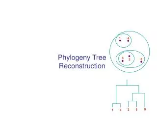
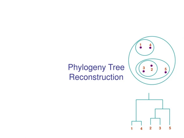
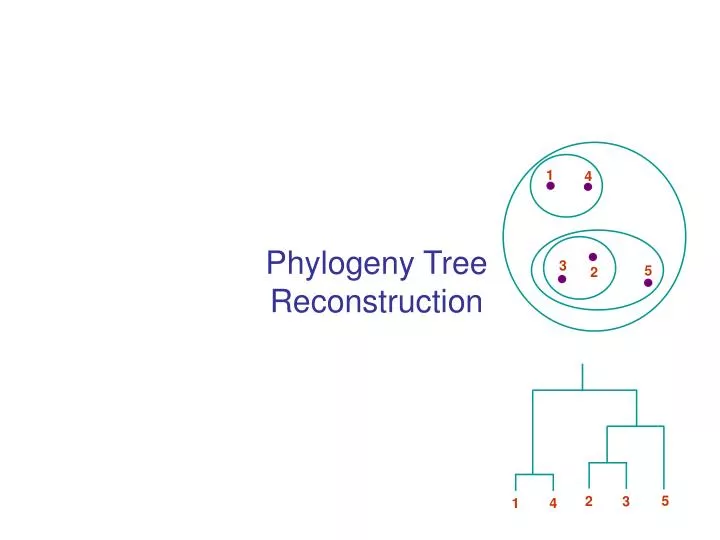
1. 4. 3. 5. 2. 5. 2. 3. 1. 4. Phylogeny Tree Reconstruction. Inferring Phylogenies. Trees can be inferred by several criteria: Morphology of the organisms Can lead to mistakes! Sequence comparison Example: Orc: A C A G T G A C G CCCC AAA C G T

E N D
1 4 3 5 2 5 2 3 1 4 Phylogeny Tree Reconstruction
Inferring Phylogenies Trees can be inferred by several criteria: • Morphology of the organisms • Can lead to mistakes! • Sequence comparison Example: Orc: ACAGTGACGCCCCAAACGT Elf: ACAGTGACGCTACAAACGT Dwarf: CCTGTGACGTAACAAACGA Hobbit: CCTGTGACGTAGCAAACGA Human: CCTGTGACGTAGCAAACGA
Neighbor-Joining 1 • Guaranteed to produce the correct tree if distance is additive • May produce a good tree even when distance is not additive Step 1: Finding neighboring leaves Define Dij = dij – (ri + rj) Where 1 ri = –––––k dik |L| - 2 Claim: The above “magic trick” ensures that Dij is minimal iffi, j are neighbors Proof: Very technical, please read Durbin et al.! Four-Point Condition: If and only if for every set of four leaves I, j, k, l, two of the distances dij + dkl, dik + djl, dil + djk are equal and larger than the third, the distances are additive and we can reconstruct the tree 3 0.1 0.1 0.1 0.4 0.4 4 2
Algorithm: Neighbor-joining Initialization: Define T to be the set of leaf nodes, one per sequence Let L = T Iteration: Pick i, j s.t. Dij is minimal Define a new node k, and set dkm = ½ (dim + djm – dij) for all m L Add k to T, with edges of lengths dik = ½ (dij + ri – rj), djk = dij – dik Remove i, j from L; Add k to L Termination: When L consists of two nodes, i, j, and the edge between them of length dij
Parsimony – What if we don’t have distances • One of the most popular methods: • GIVEN multiple alignment • FIND tree & history of substitutions explaining alignment Idea: Find the tree that explains the observed sequences with a minimal number of substitutions Two computational subproblems: • Find the parsimony cost of a given tree (easy) • Search through all tree topologies (hard)
Example: Parsimony cost of one column {A} Final cost C = 1 {A} {A, B} Cost C+=1 A B A A A A B A {B} {A} {A} {A}
Parsimony Scoring Given a tree, and an alignment column u Label internal nodes to minimize the number of required substitutions Initialization: Set cost C = 0; node k = 2N – 1 (last leaf) Iteration: If k is a leaf, set Rk = { xk[u] } // Rk is simply the character of kth species If k is not a leaf, Let i, j be the daughter nodes; Set Rk = Ri Rj if intersection is nonempty Set Rk = Ri Rj, and C += 1, if intersection is empty Termination: Minimal cost of tree for column u, = C
Example {B} {A,B} {A} {B} {A} {A,B} {A} A A A A B B A B {A} {A} {A} {A} {B} {B} {A} {B}
Traceback to find ancestral nucleotides Traceback: • Choose an arbitrary nucleotide from R2N – 1 for the root • Having chosen nucleotide r for parent k, If r Ri choose r for daughter i Else, choose arbitrary nucleotide from Ri Easy to see that this traceback produces some assignment of cost C
Example Admissible with Traceback x B Still optimal, but inadmissible with Traceback A {A, B} B A x {A} B A A B B {A, B} x B x A A B B A A A B B {B} {A} {A} {B} A x A x A A B B
Probabilistic Methods A more refined measure of evolution along a tree than parsimony P(x1, x2, xroot | t1, t2) = P(xroot) P(x1 | t1, xroot) P(x2 | t2, xroot) If we use Jukes-Cantor, for example, and x1 = xroot = A, x2 = C, t1 = t2 = 1, = pA¼(1 + 3e-4α) ¼(1 – e-4α) = (¼)3(1 + 3e-4α)(1 – e-4α) xroot t1 t2 x1 x2
Probabilistic Methods xroot • If we know all internal labels xu, P(x1, x2, …, xN, xN+1, …, x2N-1 | T, t) = P(xroot)jrootP(xj | xparent(j), tj, parent(j)) • Usually we don’t know the internal labels, therefore P(x1, x2, …, xN | T, t) = xN+1 xN+2 … x2N-1P(x1, x2, …, x2N-1 | T, t) xu x2 xN x1
Felsenstein’s Likelihood Algorithm Let P(Lk | a) denote the prob. of all the leaves below node k, given that the residue at k is a To calculate P(x1, x2, …, xN | T, t) Initialization: Set k = 2N – 1 Iteration: Compute P(Lk | a) for all a If k is a leaf node: Set P(Lk | a) = 1(a = xk) If k is not a leaf node: 1. Compute P(Li | b), P(Lj | b) for all b, for daughter nodes i, j 2. Set P(Lk | a) = b,c P(b | a, ti) P(Li | b) P(c | a, tj) P(Lj | c) Termination: Likelihood at this column = P(x1, x2, …, xN | T, t) = aP(L2N-1 | a)P(a)
Probabilistic Methods Given M (ungapped) alignment columns of N sequences, • Define likelihood of a tree: L(T, t) = P(Data | T, t) = m=1…M P(x1m, …, xnm, T, t) Maximum Likelihood Reconstruction: • Given data X = (xij), find a topology T and length vector t that maximize likelihood L(T, t)
Current popular methods HUNDREDS of programs available! http://evolution.genetics.washington.edu/phylip/software.html#methods Some recommended programs: • Discrete—Parsimony-based • Rec-1-DCM3 http://www.cs.utexas.edu/users/tandy/mp.html Tandy Warnow and colleagues • Probabilistic • SEMPHY http://www.cs.huji.ac.il/labs/compbio/semphy/ Nir Friedman and colleagues
Protein Phylogenies • Proteins evolve by both duplication and species divergence
Definition • Given N sequences x1, x2,…, xN: • Insert gaps (-) in each sequence xi, such that • All sequences have the same length L • Score of the global map is maximum • A faint similarity between two sequences becomes significant if present in many • Multiple alignments can point to elements that are conserved among a class of and therefore important in the biology of these organisms • The patterns of conservation can help us tell function of the element
Scoring Function: Sum Of Pairs Definition:Induced pairwise alignment A pairwise alignment induced by the multiple alignment Example: x: AC-GCGG-C y: AC-GC-GAG z: GCCGC-GAG Induces: x: ACGCGG-C; x: AC-GCGG-C; y: AC-GCGAG y: ACGC-GAC; z: GCCGC-GAG; z: GCCGCGAG
Sum Of Pairs (cont’d) • Heuristic way to incorporate evolution tree: Human Mouse Duck Chicken • Weighted SOP: • S(m) = k<l wkl s(mk, ml)
A Profile Representation • Given a multiple alignment M = m1…mn • Replace each column mi with profile entry pi • Frequency of each letter in • # gaps • Optional: # gap openings, extensions, closings • Can think of this as a “likelihood” of each letter in each position - A G G C T A T C A C C T G T A G – C T A C C A - - - G C A G – C T A C C A - - - G C A G – C T A T C A C – G G C A G – C T A T C G C – G G A 1 1 .8 C .6 1 .4 1 .6 .2 G 1 .2 .2 .4 1 T .2 1 .6 .2 - .2 .8 .4 .8 .4
Multiple Sequence Alignments Algorithms
Multidimensional DP Generalization of Needleman-Wunsh: S(m) = i S(mi) (sum of column scores) F(i1,i2,…,iN): Optimal alignment up to (i1, …, iN) F(i1,i2,…,iN) = max(all neighbors of cube)(F(nbr)+S(nbr))
Multidimensional DP • Example: in 3D (three sequences): • 7 neighbors/cell F(i,j,k) = max{ F(i – 1, j – 1, k – 1) + S(xi, xj, xk), F(i – 1, j – 1, k ) + S(xi, xj, - ), F(i – 1, j , k – 1) + S(xi, -, xk), F(i – 1, j , k ) + S(xi, -, - ), F(i , j – 1, k – 1) + S( -, xj, xk), F(i , j – 1, k ) + S( -, xj, - ), F(i , j , k – 1) + S( -, -, xk) }
Multidimensional DP Running Time: • Size of matrix: LN; Where L = length of each sequence N = number of sequences • Neighbors/cell: 2N – 1 Therefore………………………… O(2N LN)
Multidimensional DP • How do gap states generalize? • VERY badly! • Require 2N – 1 states, one per combination of gapped/ungapped sequences • Running time: O(2N 2N LN) = O(4N LN) Running Time: • Size of matrix: LN; Where L = length of each sequence N = number of sequences • Neighbors/cell: 2N – 1 Therefore………………………… O(2N LN) Y YZ XY XYZ Z X XZ
Progressive Alignment x • When evolutionary tree is known: • Align closest first, in the order of the tree • In each step, align two sequences x, y, or profiles px, py, to generate a new alignment with associated profile presult Weighted version: • Tree edges have weights, proportional to the divergence in that edge • New profile is a weighted average of two old profiles pxy y z pxyzw pzw w
Progressive Alignment x • When evolutionary tree is known: • Align closest first, in the order of the tree • In each step, align two sequences x, y, or profiles px, py, to generate a new alignment with associated profile presult Weighted version: • Tree edges have weights, proportional to the divergence in that edge • New profile is a weighted average of two old profiles y Example Profile: (A, C, G, T, -) px = (0.8, 0.2, 0, 0, 0) py = (0.6, 0, 0, 0, 0.4) s(px, py) = 0.8*0.6*s(A, A) + 0.2*0.6*s(C, A) + 0.8*0.4*s(A, -) + 0.2*0.4*s(C, -) Result:pxy= (0.7, 0.1, 0, 0, 0.2) s(px, -) = 0.8*1.0*s(A, -) + 0.2*1.0*s(C, -) Result:px-= (0.4, 0.1, 0, 0, 0.5) z w
Progressive Alignment x • When evolutionary tree is unknown: • Perform all pairwise alignments • Define distance matrix D, where D(x, y) is a measure of evolutionary distance, based on pairwise alignment • Construct a tree (UPGMA / Neighbor Joining / Other methods) • Align on the tree y ? z w
Heuristics to improve alignments • Iterative refinement schemes • A*-based search • Consistency • Simulated Annealing • …
Iterative Refinement One problem of progressive alignment: • Initial alignments are “frozen” even when new evidence comes Example: x: GAAGTT y: GAC-TT z: GAACTG w: GTACTG Frozen! Now clear correct y = GA-CTT
allow y to vary x,z fixed projection Iterative Refinement Algorithm (Barton-Stenberg): • For j = 1 to N, Remove xj, and realign to x1…xj-1xj+1…xN • Repeat 4 until convergence z x y
Iterative Refinement Example: align (x,y), (z,w), (xy, zw): x: GAAGTTA y: GAC-TTA z: GAACTGA w: GTACTGA After realigning y: x: GAAGTTA y: G-ACTTA + 3 matches z: GAACTGA w: GTACTGA
Iterative Refinement Example not handled well: x: GAAGTTA y1: GAC-TTA y2: GAC-TTA y3: GAC-TTA z: GAACTGA w: GTACTGA • Realigning any single yi changes nothing
A* for Multiple Alignments Review of the A* algorithm v GOAL START • Say that we have a gigantic graph G • START: start node • GOAL: we want to reach this node with the minimum path Dijkstra: O(VlogV + E) – too slow if the number of edges is huge A*: a way of finding the optimal solution faster in practice
A* for Multiple Alignments Review of the A* algorithm h(v) g(v) v GOAL Lemma Given sequences x, y, z, … The sum-of pairs score of multiple alignment M is lower (worse) than the sum of the optimal pairwise alignments Proof M induces projected pairwise alignments axy, ayz, axz, …, and Score(M) = d(axy) + d(axz) + d(ayz) +… Each of d(.) is smaller than the optimal edit distance START • g(v) is the cost so far • h(v) is an estimate of the minimum cost from v to GOAL • f(v) ≥ g(v) + h(v) is the minimum cost of a path passing by v • Expand v with the smallest f(v) • Never expand v, if f(v) ≥ shortest path to the goal found so far
A* for Multiple Alignments • Nodes: Cells in the DP matrix • g(v): alignment cost so far • h(v): sum-of-pairs of individual pairwise alignments • Initial minimum alignment cost estimate: sum-of-pairs of global pairwise alignments h(v) g(v) v GOAL START To compute h(v) For each pair of sequences x, y, Compute FR(x, y), the DP matrix of scores of aligning a suffix of x to a suffix of y Then, at position (i1, i2, …, iN), h(v) becomes the sum of (N choose 2) FR scores
Consistency zk z xi x y yj yj’
Consistency zk z Basic method for applying consistency • Compute all pairs of alignments xy, xz, yz, … • When aligning x, y during progressive alignment, • For each (xi, yj), let s(xi, yj) = function_of(xi, yj, axz, ayz) • Align x and y with DP using the modified s(.,.) function xi x y yj yj’
Some Resources Genome Resources Annotation and alignment genome browser at UCSC http://genome.ucsc.edu/cgi-bin/hgGateway Specialized VISTA alignment browser at LBNL http://pipeline.lbl.gov/cgi-bin/gateway2 ABC—Nice Stanford tool for browsing alignments http://encode.stanford.edu/~asimenos/ABC/ Protein Multiple Aligners http://www.ebi.ac.uk/clustalw/ CLUSTALW – most widely used http://phylogenomics.berkeley.edu/cgi-bin/muscle/input_muscle.py MUSCLE – most scalable http://probcons.stanford.edu/ PROBCONS – most accurate