Download
1 / 1
10 likes | 154 Views
f (x)= Cos[x]. f (x)= e x. Figure 2: Graphs showing the program’s approximation for the functions Cos[x] and e x in a uniformly spaced grid. The dashed black line is the actual Laplacian for the function and the blue line is our program’s approximation. f (x)= Cos[x]. f (x)= e x.

E N D
f(x)= Cos[x] f(x)= ex Figure 2: Graphs showing the program’s approximation for the functions Cos[x] and ex in a uniformly spaced grid. The dashed black line is the actual Laplacian for the function and the blue line is our program’s approximation. f(x)= Cos[x] f(x)= ex Figure 3: Graphs showing the program’s approximation for the functions Cos[x] and ex in a non-uniformly spaced grid. The dashed black line is the actual Laplacian for the function and the blue line is our program’s approximation. Future Work x i-2 x i-1 x i x i+1 x i+2 Automatic Generation of an Accurate Numerical Approximation of the Laplacian Operator Replace w/ Logo Alice DuVivier, Jette Petersen, David Randall, Ross Heikes CMMAP Purpose Results Mathematical Methods The goal of this project was to write a program in Mathematica to calculate the Laplacian for the twisted icosahedral grid. This will improve accuracyof the current climate models. In addition, the calculated approximation can be stored and kept for reference in future models. Both of these will decrease the cost of a particular model both in time and in the number of processors required to run the model. Finite Difference Approximation: Using Mathematica, we wrote a program to simultaneously find the Laplacian at each point on a 1D grid. This model gives promising results for a third order accurate scheme and non uniform point spacing. For both uniform grid spacing and non uniform grid spacing our approximation gives values of the Laplacian at each point that are very close to the true value when tested with a function. Figures 2 shows the uniform spaced case. Background The finite difference approximation for the second derivative at point xi using a Taylor series is as follows: The Laplacian operator, 2, is a second order differential operator. The Laplacian operator was chosen because it is frequently used in atmospheric models and relatively straightforward. However, because data on the sphere are in the form of scalar or vector values we must use finite difference quotients between values at particular points to numerically approximate the second derivative. We sum over the neighboring points about the center point. The value cj is the weight of a particular particular point in relation to the center of expansion. We solve for cj by imposing conditions dictated by the desired order of accuracy. For first order accuracy in one dimension the necessary conditions are: Figure 3 shows the non-uniformly spaced case. A twisted icosahedral grid can eliminate the so called pole problem associated with solving differential equations in spherical geometry. This scheme is essentially a 2D hexagonal grid that has been wrapped around an icosahedron representing the sphere (see figure 1). Figure 1: The twisted icosahedral grid. In the process of being wrapped about the icosahedron, the hexagonal grid cells become non-uniformly spaced and twelve hexagons are introduced into the grid. Image courtesy of Ross Heikes Future Work The weights are the solutions to the above set of linear equations. Once these weights are known the Laplacian at a particular point, i, is found by using the following straightforward formula: The algorithm for finding the Laplacian has only been written for the 1D case. We must now extend the program to a 2D hexagonal grid. Ultimately, the program will approximate the Laplacian on the twisted icosahedral grid. Once work has been completed for the Laplacian operator this method can be extended to other advection operators. To find the value of mathematical operators used in the models, such as the Laplacian, at a particular point on the grid we use weighted numerical values from the surrounding grid points. Using numerical approximation methods, we can assign weights to these neighboring points based on their distance from the point of interest and then find a weighted average for our point of interest. Developing a numerical method for approximating these non-uniform values is essential in improving models’ efficiency. By imposing conditions on the coefficients of the Taylor expansion, our program solves for these weights and then finds the Laplacian at each point on the surface to third order accuracy. Thanks to CMMAP for supporting this work.