Download
1 / 31
310 likes | 312 Views
Previous lecture. Reflectance I BRDF, BTDF, BSDF Ideal specular model Ideal diffuse (Lambertian) model Phong. Microfacet Reflectance Models. Outline. Microfacet models Diffuse Oren-Nayar Specular Torrance-Sparrow Blinn Ashikhmin-Shirley (anisotropic) Ward Schlick Lafortune’s model

E N D
Previous lecture • Reflectance I • BRDF, BTDF, BSDF • Ideal specular model • Ideal diffuse (Lambertian) model • Phong University of Texas at Austin CS395T - Advanced Image Synthesis Fall 2007 Don Fussell
Microfacet Reflectance Models University of Texas at Austin CS395T - Advanced Image Synthesis Fall 2007 Don Fussell
Outline • Microfacet models • Diffuse • Oren-Nayar • Specular • Torrance-Sparrow • Blinn • Ashikhmin-Shirley (anisotropic) • Ward • Schlick • Lafortune’s model • Two layer models University of Texas at Austin CS395T - Advanced Image Synthesis Fall 2007 Don Fussell
Microfacet Models (Text ch. 9.4) • Model surface as set of polygonal facets • Capture surface roughness effects • Microfacets can be diffuse or specular • Use facet distribution to model roughness • Statistical model of microscopic effects gives macroscopic appearance • More realistic, particularly at high incidence angles University of Texas at Austin CS395T - Advanced Image Synthesis Fall 2007 Don Fussell
Basic microfacet modeling • Surface normal distribution • How the surface normals of the facets are distributed about the macroscopic normal • Facet BRDF • Are the facets diffuse or specular? University of Texas at Austin CS395T - Advanced Image Synthesis Fall 2007 Don Fussell
Microscopic geometry • Masking – viewer can’t see a microfacet • Shadowing – light can’t see a microfacet • Interreflection – light off one facet hits another • Aim is to capture these effects as efficiently as possible University of Texas at Austin CS395T - Advanced Image Synthesis Fall 2007 Don Fussell
Oren-Nayar model (Text ch. 9.4.1) • Model facet distribution as Gaussian with s.d. (radians) • Facet BRDF is Lambertian • Resulting model has no closed form solution, but a good approximation • Sample using cosine-weighted sampling in hemisphere University of Texas at Austin CS395T - Advanced Image Synthesis Fall 2007 Don Fussell
Oren-Nayar effects Lambertian Oren-Nayar University of Texas at Austin CS395T - Advanced Image Synthesis Fall 2007 Don Fussell
Torrance-Sparrow (Text ch. 9.4.2) • Specular BRDF for facets • Arbitrary (in theory) distribution of facet normals • Additional term for masking and shadowing • Explicit Fresnel term Half vector – facet orientation to produce specular transfer n i h o University of Texas at Austin CS395T - Advanced Image Synthesis Fall 2007 Don Fussell
Torrance-Sparrow BRDF • G(o , i) handles microfacet geometry • D(h) is the microfacet orientation distribution evaluated for the half angle • Changing this changes the surface appearance • Fr(o) is the Fresnel reflection coefficient University of Texas at Austin CS395T - Advanced Image Synthesis Fall 2007 Don Fussell
Geometry term • Masking: • Shadowing: • Together: University of Texas at Austin CS395T - Advanced Image Synthesis Fall 2007 Don Fussell
Blinn’s microfacet distribution • Parameter e controls “roughness” University of Texas at Austin CS395T - Advanced Image Synthesis Fall 2007 Don Fussell
Sampling Blinn’s model (Text ch. 15.5.1) • Sampling from a microfacet BRDF tries to account for all the terms: G, D, F, cos • But D provides most variation, so sample according to D • The sampled direction is completely determined by halfway vector, h, so sample that • Then construct reflection ray based upon it • So how do we sample such a direction … University of Texas at Austin CS395T - Advanced Image Synthesis Fall 2007 Don Fussell
Blinn sampling continued • Need to sample spherical coords: , • Book has details, and probably an error on page 684 • Complication: We need to return the probability of choosing i, but we have the probability of choosing h • Simple conversion term • We need to construct the reflection direction about an arbitrary vector … University of Texas at Austin CS395T - Advanced Image Synthesis Fall 2007 Don Fussell
Arbitrary reflection • Coordinate system is not nicely aligned, so use construction University of Texas at Austin CS395T - Advanced Image Synthesis Fall 2007 Don Fussell
Anisotropic microfacet distributions • Parameters for x and y direction roughness, where x and y are the local BRDF coordinate system on the surface • Gives the reference frame for University of Texas at Austin CS395T - Advanced Image Synthesis Fall 2007 Don Fussell
Sampling anisotropic distribution • Sampling is discussed in section 15.5.2 of the text • Similar to Blinn but with different distribution • Note that there are 4 symmetric quadrants in the tangent plane • Sample in a single quadrant, then map to one of 4 quadrants • Take care to maintain stratification 0 1 1st 2nd 3rd 4th University of Texas at Austin CS395T - Advanced Image Synthesis Fall 2007 Don Fussell
Ward’s isotropic model • “the simplest empirical formula that will do the job” • Leaves out the geometry and Fresnel terms • Makes integration and sampling easier • 3 terms, plus some angular values: • d is the diffuse reflectance • s is the specular reflectance • is the standard deviation of the micro-surface slope University of Texas at Austin CS395T - Advanced Image Synthesis Fall 2007 Don Fussell
Ward’s anisotropic model • For surfaces with oriented grooves • 2 terms for anisotropy: • x is the standard deviation of the surface slope in the x direction • y is the standard deviation of the surface slope in the y direction University of Texas at Austin CS395T - Advanced Image Synthesis Fall 2007 Don Fussell
Sampling Ward’s model • Take 1 and 2 and transform to get h and h: • Only samples one quadrant, use same trick as before to get all quadrants • Not sure about correct normalization constant for solid angle measure University of Texas at Austin CS395T - Advanced Image Synthesis Fall 2007 Don Fussell
Schlick’s model (Schlick 94) • Empirical model well suited to sampling • Two parameters: • , a roughness factor (0 = Specular, 1 = Lambertian) • , an anisotropy term, (0 perfectly anisotropic, 1 = isotropic) University of Texas at Austin CS395T - Advanced Image Synthesis Fall 2007 Don Fussell
Schlick’s model • Facet Distribution: • Geometry Terms: University of Texas at Austin CS395T - Advanced Image Synthesis Fall 2007 Don Fussell
Putting it together • Term to account for inter-reflection • Not a Torrance-Sparrow model • As before, sample a half vector: • Only samples in 1 quadrant • Use trick from before • Normalization not given University of Texas at Austin CS395T - Advanced Image Synthesis Fall 2007 Don Fussell
More to it than that • Both Ward and Schlick’s original papers define complete reflectance, including diffuse and pure specular components • PBRT calls these materials, because they are simply linear sums of individual components • Schlick’s paper also includes a way to decide how to combine the diffuse, specular and glossy terms based on the roughness • Both Ward and Schlick discuss sampling from the complete distribution University of Texas at Austin CS395T - Advanced Image Synthesis Fall 2007 Don Fussell
Phong reloaded • The Phong model can be revised to make it physically reasonable – energy conserving and reciprocal • In canonical BRDF coordinate system (z axis is normal) University of Texas at Austin CS395T - Advanced Image Synthesis Fall 2007 Don Fussell
Oriented Phong • Define an orientation vector – the direction in which the Phong reflection is strongest • For standard Phong, o=(-1,-1,1) • To get “off specular” reflection, change o • Can get retro-reflection, more reflection at grazing, etc. University of Texas at Austin CS395T - Advanced Image Synthesis Fall 2007 Don Fussell
Lafortune’s model (Text ch. 9.5) • A diffuse component plus a sum of Phong lobes • Allow all parameters to vary with wavelength • Lots of parameters, 12 for each lobe, so suited for fitting to data • It’s reasonably easy to fit • Parameters for many surfaces are available University of Texas at Austin CS395T - Advanced Image Synthesis Fall 2007 Don Fussell
Lafortune’s clay University of Texas at Austin CS395T - Advanced Image Synthesis Fall 2007 Don Fussell
Sampling Lafortune • First choose a lobe (or diffuse) • Could be proportional to lobe’s contribution to outgoing direction • But that might be expensive • Then sample a direction according to that lobe’s distribution • Just like sampling from Blinn’s microfacet distribution, but sampling the direction directly University of Texas at Austin CS395T - Advanced Image Synthesis Fall 2007 Don Fussell
Two-layer models (Text chs. 9.6 and 15.5.3)) • Captures the effects of a thin glossy layer over a diffuse substrate • Common in practice – polished painted surfaces, polished wood, … • Glossy dominates at grazing angles, diffuse dominates at near-normal angles • Don’t need to trace rays through specular surface to hit diffuse University of Texas at Austin CS395T - Advanced Image Synthesis Fall 2007 Don Fussell
Fresnel blend model University of Texas at Austin CS395T - Advanced Image Synthesis Fall 2007 Don Fussell