Download
1 / 15
150 likes | 155 Views
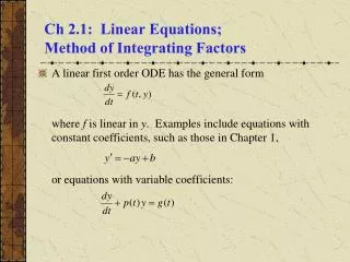
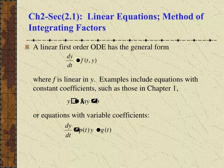
Ch2-Sec(2.1): Linear Equations; Method of Integrating Factors. A linear first order ODE has the general form where f is linear in y . Examples include equations with constant coefficients, such as those in Chapter 1, or equations with variable coefficients:. Constant Coefficient Case.

E N D
Ch2-Sec(2.1): Linear Equations; Method of Integrating Factors • A linear first order ODE has the general form where f is linear in y. Examples include equations with constant coefficients, such as those in Chapter 1, or equations with variable coefficients:
Constant Coefficient Case • For a first order linear equation with constant coefficients, recall that we can use methods of calculus to solve:
Variable Coefficient Case: Method of Integrating Factors • We next consider linear first order ODEs with variable coefficients: • The method of integrating factors involves multiplying this equation by a function (t), chosen so that the resulting equation is easily integrated.
Example 2: Integrating Factor (1 of 2) • Consider the following equation: • Multiplying both sides by (t), we obtain • We will choose (t) so that left side is derivative of known quantity. Consider the following, and recall product rule: • Choose (t) so that
Example 2: General Solution (2 of 2) • With (t) = et/2, we solve the original equation as follows:
Method of Integrating Factors: Variable Right Side • In general, for variable right side g(t), the solution can be found as follows:
Example 3: General Solution (1 of 2) • We can solve the following equation using the formula derived on the previous slide: • Integrating by parts, • Thus
Example 3: Graphs of Solutions (2 of 2) • The graph shows the direction field along with several integral curves. If we set C = 0, the exponential term drops out and you should notice how the solution in that case, through the point (0,-7/4), separates the solutions into those that grow exponentially in the positive direction from those that grow exponentially in the negative direction..
Method of Integrating Factors for General First Order Linear Equation • Next, we consider the general first order linear equation • Multiplying both sides by (t), we obtain • Next, we want (t) such that '(t) = p(t)(t), from which it will follow that
Integrating Factor for General First Order Linear Equation • Thus we want to choose (t) such that '(t) = p(t)(t). • Assuming (t) > 0, it follows that • Choosing k = 0, we then have and note (t) > 0 as desired.
Solution forGeneral First Order Linear Equation • Thus we have the following: • Then
Example 4: General Solution (1 of 2) • To solve the initial value problem first put into standard form: • Then and hence
Example 4: Particular Solution (2 of 2) • Using the initial condition y(1) = 2 and general solution it follows that • The graphs below show solution curves for the differential equation, including a particular solution whose graph contains the initial point (1,2). Notice that when C=0, we get the parabolic solution (shown) and that solution separ- ates the solutions into those that are asymptotic to the positive versus negative y-axis. (1,2)
Example 5: A Solution in Integral Form (1 of 2) • To solve the initial value problem first put into standard form: • Then and hence
Example 5: A Solution in Integral Form (2 of 2) • Notice that this solution must be left in the form of an integral, since there is no closed form for the integral. • Using software such as Mathematica or Maple, we can approximate the solution for the given initial conditions as well as for other initial conditions. • Several solution curves are shown.