Download
1 / 31
310 likes | 425 Views
Matrix Eigensystem Tutorial For Parallel Computation. High Performance Computing Center (HPC) http://www.hpc.unm.edu. Outline. Outline Continued. Outline Continued. Main Purpose Of This Tutorial.

E N D
Matrix Eigensystem Tutorial For Parallel Computation High Performance Computing Center (HPC) http://www.hpc.unm.edu
Main Purpose Of This Tutorial • Short and concise complement to the ScaLAPACK Users’ Guide and Tutorial and other package documentation • To explain the problems a user encounters using ScaLAPACK on a typical Linux cluster • To provide solutions for the typical problems
The Assumptions Made About The Users Of This Tutorial • The parallel eigensystem software is installed in an appropriate location in the machine and user needs to be aware of that location • Users are assumed to be familiar with: • The definition of the matrix eigensystem problem • Using an editor • The Fortran programming language • Program compilation and makefiles • Debugging a parallel program • Setting the necessary environment variables on a specific machine to submit and run a parallel program
Important Points To Be Noted • The application code should be compiled with the same compiler that the parallel eigensystem library is built with. Otherwise, your driver code may not compile and/or link correctly, or may not produce the correct results • Later slides will be provided on the topics of: • How to create a Makefile (Specific to the Linux) • How to submit and run a parallel job on Linux system using PBS
SCALAPACK PBLAS LAPACK BLACS BLAS Organization Of ScaLAPACK • Organization • A library of parallel math procedures • Components of ScaLAPACK (dependency graph) • PBLAS: Parallel BLAS (Basic Linear Algebra Subroutines) • BLACS: Parallel Communication • LAPACK: Serial linear algebra computation • BLAS: Serial BLAS • Note: • The compilation and linking of the users’ program must provide access to these libraries • In the linking process, the more general libraries (highest in the dependency graph) should be first with the BLAS last
References To ScaLAPACK • ScaLAPACK Users’ Guide (published by SIAM Press) • Parallel Mathematical Libraries (http://webct.ncsa.uiuc.edu:8900) • Describes the structure of ScaLAPACK • Provides a guide for using ScaLAPACK routines • Highlights processor grid creation and ScaLAPACK data distribution; this tutorial assumes knowledge of this topic • Provides a working example for matrix-vector multiplication, using ScaLAPACK • ScaLAPACK Tutorial (http://www.netlib.org/scalapack/tutorial) • Highlights structure, design, content, performance of ScaLAPACK and other libraries (EISPACK, LINPACK, LAPACK, BLAS, BLACS, PBLAS, ATLAS) • Provides examples of calls to ScaLAPACK and other library routines • ScaLAPACK Example Programs (http://www.netlib.org/scalapack/examples) • Provides working examples for solving symmetric, Hermitian, generalized symmetric, and generalized Hermitian eigenproblems
Brief Definition Of Eigensystem • Right eigensystem • To compute the non-zero right eigenvector (x) of matrix A corresponding to the eigenvalue λ, satisfying the equation A x = λ x • Left eigensystem • To compute the non-zero left eigenvector (x) of matrix A corresponding to the eigenvalue λ, satisfying the equation xT A = λ xT
Why You Need To Study This Tutorial Before Calling ScaLAPACK Routines • Calling an inappropriate routine for your eigenproblem may create very inaccurate results • For example, don’t solve the symmetric eigenproblem with the general matrix eigenproblem routines • Some important concerns: • The type of input matrix A (complex, hermitian, symmetric, banded, dense, sparse, …) • The data storage and distribution (determined by the user or by the library) • Picking the correct algorithm for the following cases • Standard problem (Ax = λx) • Generalized eigensystems (Ax = λBx, ABx = λx) • Symmetric and non-symmetric eigensystem problems • Singular values and pseudo-inverses • Least squares problem (may be)
Generic Steps In Solving The Eigenvalue Problem • Reduce the original matrix to a condensed form by similarity transformations • Kinds of condensed form: • Reduce a symmetric matrix to tridiagonal form • Reduce a non-symmetric matrix to Hessenberg form, and the Hessenberg form to the Schur form • Reduce a rectangular matrix to bidiagonal form to compute a singular value decomposition • Compute the eigensystem of the condensed form • Transform the eigenvectors of the condensed form back to the original matrix eigenvectors. The eigenvalues of the condensed form are the same as the eigenvalues of the original matrix
Data-type S: Real (Single precision) D: Double precision C: Complex Z: Double complex (or Complex*16) Note: The list is shown for the Fortran language and Fortran is not case sensitive Matrix-type SY: SYmmetric (real) HE: HErmitian (complex) OR: ORthogonal (real) UN: UNitary (complex) GE: GEneral (nonsymmetric, and may be rectangular) TR: Tridiagonal ST: Symmetric Tridagonal PO: POsitive definite Data-type And Matrix-type Designators In The ScaLAPACK Routines
Classification Of ScaLAPACK Routines • Routines in ScaLAPACK are classified as: Driver, Computational, and Auxiliary routines • Driver routines: • Simple Driver • A single driver computes all the eigenvalues and eigenvectors of a matrix • Expert Driver • An expert driver computes all or a selected subset of the eigenvalues and eigenvectors of a matrix • Computational routines • More than one routine is necessary to complete the eigensystem computations • Auxiliary routines • Compute certain subtask or common low-level computations (e.g, max, min, abs routines)
ScaLAPACK Generic Naming Conventions For Drivers And Computational Routines • SCALAPACK naming system is essentially the same as LAPACK with P added in the beginning of the name (P stands for parallel) • The general form of names of Drivers and Computational routines are as follows (includes at most 7 characters with only 2 ZZZ characters for the Driver routines) Pxyyzzz Symbols represent: P: Parallel x: Datatype designator such as S: real, D: double, ... yy: Matrix type designator such as: GE: general, SY: symmetric, …, or LA: auxiliary routine zzz: Computation type such as: EV: eigenvalues and eigenvectors As an example, PSSYEV is the driver for the parallel (P) eigensystem solver for a single (S) precision symmetric (SY) matrix which finds all eigenvalues (E) and eigenvectors (V)
ScaLAPACK Generic Naming Convention For Auxiliary Routines • In the Auxiliary routines • A similar naming scheme as the previous slide except that YY is replaced with LA • Exceptions: • The non-blocked version of the blocked algorithms have the character 2 instead of a letter at the end (e.g., PSGETF2 is the unblocked version of PSGETRF) • A few routines which are regarded as extensions to BLAS have similar names to the BLAS routines
Naming Convention For The Driver Routines • Computational part (ZZZ) in Driver routine names: • Simple Driver • ZZZ string is EV (EigenValues & eigenVectors) • Expert Driver • Computes all or a selected subset of the eigenvalues and eigenvectors • ZZZ string is EVX • Computes the solution to the Generalized Symmetric Definite Eigenproblems • zzz string is with GVX
Naming Convention For The Computational Routines • In the Computational routines: ZZZ is replaced with several acronyms depending on the matrix-type as described below • Symmetric eigenproblem • Computes eigenvalues and eigenvectors of real-symmetric or complex-Hermitian matrix A • Steps in computation • When reducing A to tridiagonal form, the zzz string is TRD, meaning Tridiagonal ReDuction • When computing eigenvalues/eigenvectors of a tridigonal matrix, the string zzz may be EIG, meaning computation of eigensystem
Naming Convention For The Computational Routines Continued • Nonsymmetric Eigenproblems • Compute eigenvalues/vectors of general matrix A • Steps in computation • When reducing matrix A to upper Hessenberg form, the string ZZZ is HRD • When reducing upper Hessenberg matrix to Schur form and computing eigenevalues of the Schur form, the string ZZZ is HQR • When computing eigenvectors of the Schur form and transforming them back to the eigenvectors of matrix A, the string ZZZ is EVC • Note: An explanation of an intermediate step and more guides are provided in succeeding sections • Generalized Symmetric Definite Eigenproblems • Generalized Symmetric Definite Eigenproblems is defined in the succeeding sections • Steps in Computing eigenvalues/vectors of generalized eigenvalue problems • When reducing the problem to a standard symmetric eigenproblem, the string ZZZ is GST, meaning Generalized Symmetric definite Transformation • Compute eigenvalues/vectors with routines provided for symmetric eigenproblems
How To Pick The Appropriate Driver To Solve A Specific Eigensystem In ScaLAPACK • Driver routines • Solve a complete problem • Limited number of these routines are available • There is not a Driver routine for every problem • Standard symmetric eigenvalue problem • Solves Az = λz (A = AT , A is real) for symmetric eigensystem problem • call PxSYEV/PxSYEVX subroutines • P: Parallel, x: datatype (S, D), SY: Symmetric, EV: all eigenvalue/vector, X: Expert routine • Solves Az = λz (A = AH , A is complex)for Hermitian eigensystem problem • call PxHEEV/PxHEEVX subroutines • P: Parallel, x: datatype (C, Z), HE: Hermitian, EV: all eigenvalue/vector, X: Expert routine
How To Pick The Appropriate Driver Routines To Solve A Specific Eigensystem In ScaLAPACK Continued • Generalized Symmetric Definite Eigenproblem • Solves Az = λBz, ABz = λz, BAz = λz, where λ is real, A is SY/HE, B is symmetric positive definite • Use PxyyGVX Driver routine • P: Parallel, x:datatype(S,C,D,Z), yy: matrix-type (real-Symmetric (SY), complex-Hermitian (HE)), G: Generalized, V: EigenVector, X: Expert routine • Nonsymmetric matrix • No expert routine is available
How To Pick The Appropriate Computational Routine For Eigensystem In ScaLAPACK • Computational Routines • Symmetric Eigenproblems • Compute eigenvalues/vectors of Az = λz, A is real-symmetric (SY) or complex-Hermitian (HE) • First, reduce A to a tridiagonal form T • The decomposition has the forms of A = Q T QT or A = Q T QH • Use PxSYTRD or PxHETRD subroutine respectively • Second, compute eigenvalues/vectors of T with the following 3 possible subroutines: • To find the Eigenvalues/vectors via look-ahead QR algorithm, use XSTEQR2 • To find the Eigenvalues of T via bisection, use PxSTEBZ subroutine • To find the Eigenvectors of T by inverse iteration, use PxSTEIN • Third, to transform the eigenvectors of T back to eigenvectors of A, use PxORMTR or PxUNMTR subroutine, Multiply T (TRiangular) by ORthogonal or UNitary matrix Q
How To Pick The Appropriate Computational Routines For Eigensystem In ScaLAPACK Continued • Nonsymmetric eigenproblems • Compute all eigenvalues of λ and right eigenvectors v and/or left eigenvectors u in the following equations Av = λv or uHA = λuH • First, reduce the general matrix A to upper Hessenberg form H (A = QHQT or A = QHQH) • Call PxGEHRD subroutine • P: Parallel, x: datatype (S,D,C,Z), GE: GEneral, H: Hessenberg, RD: Reduced • Second, call PxORMHR or PxUNMHR to generate the orthogonal/unitary matrix Q • Third, reduce H to Schur form T (H = STST or H = STSH), where S represents the Schur vectors of H • Call auxiliary routine PxLAHQR, x: datatype (S,D,C,Z) • Fourth, call PxTREVC to compute the eigenvectors of T and transform them back to the coordinate space of the original matrix A, x: datatype (C,Z) H Q
How To Pick The Appropriate Computional Routines For Eigensystem In ScaLAPACK Continued • Generalized Symmetric Definite Eigenproblems • Compute the eigenvalues/vectors of Az = λBz, ABz = λz, BAz = λz, where A and B are real-symmetric/Complex-Hermitian, B is positive definite • Reduce each problem to a standard symmetric eigenvalues problem, using a Cholesky factorization of B • Given A and the factored B, use routine PxyyGST to overwrite A with C representing the standard problem Cy = λy with the same eigenvalues and related eigenvectors • P: Parallel, x: datatype (S,D,C,Z), yy: (SY, HE), G: Generalized ST: Symmetric definite Transformation • Solve the standard form with one of the routines provided for the symmetric eigenproblem shown the previous (slide 21)
Theory Of Computing Eigenvalues/Eigenvectors Of Non-symmetric-Complex Matrix • The process (theory): Only the process for the right eigenvectors is described. A similar discussion for the left eigenvector is provided in an Appendix to these slides A x = λ x H is the Hessenberg form of A and Q is unitary:A = QHQH T is the Schur form of H and Z is a unitary:H= ZTZH Replace A and H: multiply by (QZ)-1: QZTZHQH x = λx T(QZ)H x = λ(QZ)-1 x compare toTY = λY(Y is the right eigenvector of T) Y = (QZ)H x => x = QZY • As a result, to compute x, we need to compute Y (the right eigenvector of T), and then multiply by the product of QZ • The complete description of the routines which implement the above theory is described in the following slides
H A Q Converting The Theory Of Computing Eigenvalues/Eigenvectors Of Non-symmetric-Complex Matrix To Code • The essence of a sample code is provided in slide (??). • A complete working sample code is provided in slide (??). • STEP 1: Call zgehrd subroutine to reduce the input matrix A to Hessenberg form (A = QHQH) • The Hessenberg form (H) is stored in the upper part of the input matrix A. Part of the unitary matrix Q is stored below the subdiagonal of A. The rest of Q is stored in the vector TAU. => zgehrd
Converting The Theory Of Computing Eigenvalues/Eigenvectors Of Non-symmetric-Complex Matrix To Code Continued • STEP 2: Call the subroutine zunghr to generate unitary matrix Q from the encoding of Q which is computed in the previous routine (zgehrd) and was stored in A and TAU • The input matrix A is overwritten by this routine with the unitary matrix Q (The name Q is used instead of A in the sample code)
Converting The Theory Of Computing Eigenvalues/Eigenvectors Of Non-symmetric-Complex Matrix To Code Continued • STEP 3: Call the suboutine zhseqr to perform the following 3 operations: • Compute eigenvalues of upper Hessenberg matrix, which was computed by zgehrd and was stored in the upper part of matrix A (or H in the sample code) • Store the eigenvalues in array W • Compute Schur form (upper triangular form) of matrix H (Hessenberg form) • Store the upper triangular form in matrix H • Compute the product of QZ (the unitary matrix Q was generated by zunghr), and Z, the unitary matrix that transform H to the uppper triangular Schur form • Store the product QZ in matrix Z Note: The eigenvalues of the input matrix A, the Hessenberg form of A, and the Schur form of A are same because these matrices are similar (in the mathematical sense).
Converting The Theory Of Computing Eigenvalues/Eigenvectors Of Non-symmetric-Complex Matrix To Code Continued • STEP 4: Call ztrevc subroutine to perform 2 tasks: • Compute the eigenvectors of Schur form which was stored in matrix H by the previous subroutine, zhseqr • Transform these eigenvectors back to the space of original matrix A • Store the eigenvectors of the original matrix in matrix VR (for right eigenvectors)
Sample Code To Calculate The Right-Eigenvectors in LAPACK ! A is a non-Hermitian-complex input matrix call ZGEHRD(N, ILO, IHI, A, LDA, TAU, WORK, LWORK, INFO) H = A Q = A call ZUNGHR(N, ILO, IHI, Q, LDA, TAU, WORK, LWORK, INFO) call ZHSEQR(‘S’, ‘V’, N, ILO, IHI, H, LDA, W, Q, LDA, WORK, LWORK, INFO) VR = Q call ZTREVC(‘R’, ‘B’, SELECT, N, H, LDA, VL, LDA, VR, LDA, MM, M, WORK, RWORK, INFO)
Left Eigenvectors Of Non-symmetric-complex Matrix • The left eigenvector computation is slight modification of the computation for right eigenvector as follows xH A = λ xH The matrix H is the Hessenberg form of A and Q is unitary:A = QHQH The matrixT is the upper triangular Schur form of H and Z is a unitary:H= ZTZH Replace A and H: Right multiply by (QZ): xHQZTZHHQH = λxH xHQZT = λxH(QZ)andcompare toYHT = λYH YH = xHQZ=> xH = YHQHZH or x = QZY • As a result, to compute x, need to compute Y (left eigenvector of T), and then multiply by the product of QZ • The complete description of the subroutines which implement the above theory is described in the following slides