Download
1 / 35
350 likes | 362 Views
Distributed Databases. Chapter 16. Two Types of Applications that Access Distributed Databases. The application accesses data at the level of SQL statements.

E N D
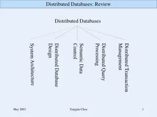
Distributed Databases Chapter 16
Two Types of Applications that Access Distributed Databases • The application accesses data at the level of SQL statements. • Example: company has nationwide network of warehouses, each with its own database; a transaction can access all databases using their schemas • The application accesses data at a database using only stored procedures provided by that database. • Example: purchase transaction involving a merchant and a credit card company, each providing stored subroutines for its subtransactions
Optimizing Distributed Queries • Only applications of the first type can access data directly and hence employ query optimization strategies. • These are the applications we consider in this chapter.
Some Issues • How should a distributed database be designed? • At what site should each item be stored? • Which items should be replicated and at which sites? • How should queries that access multiple databases be processed? • How do issues of query optimization affect query design?
Why Might Data Be Distributed • Data might be distributed to minimize communication costs or response time. • Data might be kept at the site where it was created so that its creators can maintain control and security. • Data might be replicated to increase its availability in the event of failure or to decrease response time.
Application Designer’s View of a Distributed Database • Designer might see the individual schemas of each local database -- called a multidatabase -- in which case distribution is visible. • Can be homogeneous (all databases from one vendor) or heterogeneous (databases from different vendors) • Designer might see a single global schema that integrates all local schemas – a view -- in which case distribution is hidden. • Designer might see a restricted global schema, which is the union of all the local schemas. • Supported by some vendors of homogeneous systems
Views of Distributed Data • (a) Multidatabase with local schemas • (b) Integrated distributed db with global schema
Multidatabases • Application must explicitly connect to each site. • Application accesses data at a site using SQL statements based on that site’s schema. • Application may have to do reformating in order to integrate data from different sites. • Application must manage replication. • Know where replicas are stored and decide which replica to access
Global and Restricted Global Schemas • Middleware provides integration of local schemas into a global schema • Application need not connect to each site • Application accesses data using global schema • Need not know where data is stored – location transparency • Global joins are supported • Middleware performs necessary data reformating • Middleware manages replication – replication transparency
Fragmentation • Data can be distributed by storing individual tables at different sites • Data can also be distributed by decomposing a table and storing portions at different sites – called Fragmentation • Fragmentation can be horizontal or vertical
Horizontal Fragmentation • Each fragment, Ti , of table T contains a subset of the rows and each row is in exactly one fragment: • Ti = Ci (T) • T = Ti • Horizontal fragmentation is lossless
Horizontal Fragmentation • Example: An Internet grocer has a relation describing inventory at each warehouse Inventory(StockNum, Amount, Price, Location) • It fragments the relation by location and stores each fragment locally: rows with Location = `Chicago` are stored in the Chicago warehouse in a fragment • Alternatively, it can use the schema • Inventory_ch(StockNum, Amount, Price, Location) Inventory_ch(StockNum, Amount, Price)
Vertical Fragmentation • Each fragment, Ti, of T contains a subset of the columns, each column is in at least one fragment, and each fragment includes the key: • Ti = attr_listi (T) • T = T1 T2 ….. Tn • Vertical fragmentation is lossless • Example: The Internet grocer has a relation Employee(SSnum, Name, Salary, Title, Location) • It fragments the relation to put some information at headquarters and some elsewhere: Emp1(SSnum, Name, Salary) -- at headquarters Emp2(SSnum, Name, Title, Location) -- elsewhere
Mixed Fragmentation • Combinations of horizontal and vertical fragmentation • Horizontal then vertical • Vertical then horizontal Exp: After vertical fragmentation to Emp1(Ssnum, Name, Salary, Location) Emp2(Ssnum, Name, Salary, Location) the company can do a horizontally fragmentation
Derived Horizontal Fragmentation Inventory(StockNum, Amt, Price, WareHN) Warehouse(WareHN, Cap, Add, Location) One DB in each city => good for a horizontal fragmentation of Inventory BUT: Location is not an attribute of Inventory => Do the natural join then create the horizontal fragmentation; when store data, remove the location attribute
Replication • One of the most useful mechanisms in distributed databases • Increases • Availability • If one replica site is down, data can be accessed from another site • Performance: • Queries can be executed more efficiently because they can access a local or nearby copy • Updates might be slower because all replicas must be updated
Replication Example • Internet grocer might have relation Customer(CustNum, Address, Location) • Queries are executed at • Headquarters to produce monthly mailings • A warehouse to obtain information about deliveries • Updates are executed at • Headquarters when new customer registers and when information about a customer changes
Example (con’t) • Intuitively it seems appropriate to • Store complete relation at headquarters • Horizontally fragment a replica of the relation and store a fragment at the corresponding warehouse site • Each row is replicated: one copy at headquarters, one copy at a warehouse
Example (con’t): Performance Analysis • We consider three alternatives: • Store the entire relation at the headquarters site and nothing at the warehouses (no replication) • Store the fragments at the warehouses and nothing at the headquarters (no replication) • Store entire relation at headquarters and a fragment at each warehouse (replication)
Example (con’t): Performance Analysis - Assumptions • To evaluate the alternatives, we estimate the amount of information that must be sent between sites. We make the following assumptions • The Customer relation has 100,000 rows • The headquarters mailing application sends each customer one mailing a month • 500 deliveries are made each day, and a single row must be read for each delivery • There are 100 new customers a day (and changes to customer information occur negligibly often)
Example: The Evaluation • Entire relation at headquarters, nothing at warehouses • 500 tuples per day from headquarters to warehouses for deliveries • Fragments at warehouses, nothing at headquarters • 100,000 tuples per month from warehouses to headquarters for mailings (3,300 tuples per day, amortized) • 100 tuples per day from headquarters to warehouses for new customer registration • Entire relation at headquarters, fragments at each warehouse • 100 tuples per day from headquarters to warehouses for new customer registration
Example: Conclusion • Replication seems best, but there might be other considerations • If no data stored at warehouses, the time to handle deliveries might suffer because of the remote access (probably not important) • If no data is stored at headquarters, the monthly mailing requires that 100,000 rows be transmitted in a single day, which might clog the network • If we replicate, the time to register a new customer might suffer because of the remote update • But this update can be done by a separate transaction after the registration transaction commits (asynchronous update)
Query Planning • Systems that support a global schema contain a global query optimizer, which analyzes each global query and translates it into an appropriate sequence of steps to be executed at each site • In a multidatabase system, the query designer must manually decompose each global query into a sequence of SQL statements to be executed at each site • Thus a query designer must be her own query optimizer
Global Query Optimization • A familiarity with algorithms for global query optimization helps the application programmer in designing • Global queries that will execute efficiently for a particular distribution of data • Algorithms for efficiently evaluating global queries in a multidatabase system • The distribution of data that will be accessed by global queries
Planning Global Joins • Suppose an application at site A wants to join tables at sites B and C. Two straightforward approaches • Transmit both tables to site A and do the join there • The application explicitly tests the join condition • This approach must be used in multidatabase systems • Transmit the smaller of the tables, e.g. the table at site B, to site C; execute the join there; transmit the result to site A • This approach might be used in a homogenous distributed database system
Global Join Example • Site B Student(Id, Major) • Site C Transcript(StudId, CrsCode) • Application at Site A wants to compute join with join condition Student.Id = Transcript.StudId
Assumptions • Lengths of attributes • Id and StudId: 9 bytes • Major: 3 bytes • CrsCode: 6 bytes • Student has 15,000 tuples, each of length 12 bytes • 5000 students are registered for at least 1 course and, on average, each is registered for 4 courses • Thus Transcript has 20,000 tuples each of length 15 bytes
Comparison of Alternatives • If we send both tables to site A to perform the join, we have to send 480,000 bytes 15,000*12 + 20,000*15 • If we send the smaller table, Student, from site B to site C, compute the join there, and then send the result to Site A, we have to send 540,000 bytes 15,000*12 + 20,000*18 • Thus alternative 1 is better
Another Alternative: Semijoin • At site C, compute a table, P, that is the projection of Transcript on StudId; send P to site B. • P contains Ids of students registered for at least 1 course • Student tuples having Ids not in P do not contribute to join • At site B, form the join of Student with P using the join condition; send the result, Q, to site C • Q contains tuples of Student corresponding to students registered for at least 1 course • Q is the semijoin; it is the set of all Student tuples that will participate in the join • At site C compute the join of Transcript with Q using the join condition; send the result to A
Comparision with Previous Alternatives • In step 1, we send 45,000 bytes 5,000*9 • In step 2, we send 60,000 bytes 5,000*12 • In step 3, we send 360,000 bytes 20,000*18 • In total, we send 465,000 bytes 45,000 + 60,000 + 360,000 • Semijoin is the best of the three alternatives
Definition of Semijoin • The semijoin of two relations, T1 and T2, based on a join condition is the projection over the columns of T1 of the join of T1 and T2 • In other words, the semijoin consists of the tuples in T1 that participate in the join with T2 attributes(T1)(T1join_condition T2)
Using the Semijoin • To compute the join of T1 and T2 based on a join condition, we first compute the semijoin, Q, and then join Q with T2 attributes(T1)(T1join_condition T2) join_condition T2
Queries that Involve Joins and Selections • Suppose the Internet grocer relation Employee is vertically fragmented as Emp1(SSnum, Name, Salary) at Site B Emp2(SSnum, Title, Location) at Site C • A query at site A wants the names of all employees with Title = ‘manager’ and Salary > ‘20000’ • Solution 1: do join before selection – i.e., evaluate • A semijoin is not helpful because all tuples of each table must be brought together to form join Name (Title=‘manager’ AND Salary>’20000’ (Emp1 Emp2))
Queries that Involve Joins and Selections • Solution 2: Do selections before the join: evaluate • At site B, select all tuples from Emp1 satisfying Salary > ‘20000’; call the result R1 • At site C, select all tuples from Emp2 satisfying Title = ‘manager’; call the result R2 • At some site to be determined by minimizing communication costs, perform the join of R1 and R2, project on the result using Name; send result to site A • In multidatabase join must be performed at Site A, but communication costs are reduced because only “selected” data needs to be sent Name((Salary>’20000’(Emp1)) (Title=‘manager’(Emp2)))
Choices of the Distributed Database Application Designer • Place tables at different sites • Fragment tables in different ways and place fragments at different sites • Replicate tables or data within tables (i.e. denormalize) and place replicas at different sites • In multidatabase systems, do manual “query optimization”: choose an optimal sequence of SQL statements to be executed at each site