Download
1 / 33
330 likes | 338 Views
This article explores the concept of adding functions in finite precision using the Fast Multipole algorithm. It discusses the exclusive sum problem and presents different algorithms and data structures for efficient computations. The article also covers algorithms for exclusive sum in various topologies and provides pseudocode and examples.

E N D
Fast Multipole: It's All About Adding Functions in Finite Precision Alan Edelman Per-Olof Persson MIT: Dept of Mathematics, Computer Science Artificial Intelligence Laboratory University of Maryland, College Park April 27, 2004
Exclusive Sum Problem • Given vector x compute “exclusive sum”: yi = ∑j≠ixj • Example: x=[ 1 2 3 4 5 6 7 8] y=[35 34 33 32 31 30 29 28] • Students quickly think of “sum(x)-x” • Now impose NO SUBTRACTION rule
10 26 3 7 11 15 Tree algorithm for exclusive sum 1 2 0 36 3 10 26 33 29 25 21 3 7 11 15 4 35 34 33 32 31 30 29 28 1 2 3 4 5 6 7 8 5 6 Up the tree: Pairwise Adds Down the tree: Sibling Swap + Parent 7 8
10 26 3 7 11 15 Parallel Prefix Like Algorithm 1 2 0 36 3 26 10 10 26 33 29 25 21 3 7 11 15 4 35 34 33 32 31 30 29 28 1 2 3 4 5 6 7 8 5 6 Up the tree: Pairwise Adds Down the tree: Sibling Swap + Parent 7 8 Adds may be done in parallel
10 26 3 7 11 15 Parallel Exclusive Prefix Algorithm 1 2 0 36 3 0 10 10 26 0 3 10 21 3 7 11 15 4 0 1 3 6 10 15 21 28 1 2 3 4 5 6 7 8 5 Down the tree: if right : add left if left : add 0 + Parent 6 Up the tree: Pairwise Adds 7 8 Adds may be done in parallel
The prefix operator yk=∑i=1xi k “Parallel Prefix” goes back to 1800’s: Babbage, carry, look-ahead addition
Simple algorithm for exclusive sum x=[ 1 2 3 4 5 6 7 8] • Compute directly: exclusive_prefix_sum=[ 0 1 3 6 10 15 21 28] exclusive_suffix_sum=[35 33 30 26 21 15 8 0 ] • Vector sum: y=[35 34 33 32 31 30 29 28]
The Algorithm Menu • Direction of Summation • Prefix • Suffix • Bidirectional • Exclusions • Inclusive • Exclusive • Neighborhood Exclusive • Topology • Line (1d) • Plane (2d) • Space (3d) • Circle, sphere, manifolds, … • Data Structure • Direct • Hierarchical • Function Representation • Exact • Multipole • Interpolation
The Algorithm Menu • Direction of Summation • Prefix • Suffix • Bidirectional • Exclusions • Inclusive • Exclusive • Neighborhood Exclusive • Topology • Line (1d) • Plane (2d) • Space (3d) • Circle, sphere, manifolds, … • Data Structure • Direct • Hierarchical • Function Representation • Exact • Multipole • Interpolation 2d FMM: 1c+2c+3b+4b+5b ParPrefix:1a+2a+3a+4b+5a
The Algorithm Menu • Direction of Summation • Prefix • Suffix • Bidirectional • Exclusions • Inclusive • Exclusive • Neighborhood Exclusive
The Algorithm Menu • Direction of Summation • Prefix • Suffix • Bidirectional • Exclusions • Inclusive • Exclusive • Neighborhood Exclusive Pseudocode:
The Algorithm Menu • Direction of Summation • Prefix • Suffix • Bidirectional • Exclusions • Inclusive • Exclusive • Neighborhood Exclusive
The Algorithm Menu • Direction of Summation • Prefix • Suffix • Bidirectional • Exclusions • Inclusive • Exclusive • Neighborhood Exclusive
The Algorithm Menu • Direction of Summation • Exclusions • Topology • Data Structure • Function Representation • Discrete algorithms cover 1,2,3 and 4 • Item 5 needs • Functions • Discrete Representation of Functions • Addition on this representation
Exclude (Numbers or functions) MATLAB: Tree algorithm expressed recursively >> exclude([1 2 3 4 5 6 7 8]) ans = 35 34 33 32 31 20 29 28 >> exclude([1/(t-1) 1/(t-2)1/(t-3)1/(t-4)]) ans = [1/(t-2)+1/(t-3)+1/(t-4), 1/(t-1)+1/(t-3)+1/(t-4), 1/(t-4)+1/(t-1)+1/(t-2), 1/(t-3)+1/(t-1)+1/(t-2)]
Function Representation:The analog of rounding • Interpolate • Number of points • Locations of points • Approximate • L2 (least squares) • L∞ (“Remez”) • Polynomials: f(x)=∑0 ≤ k <p ak(x-c)k • Truncated Multipole Series: f(x)=∑1 ≤ k ≤ p ak/(x-c)k • Virtual Charges: f(x)=∑1 ≤ k ≤ p ak/(x-xk)
Function Representation:The analog of rounding f(x)=1/(x-0.75)
Virtual Charges f(x)=∑1 ≤ k ≤ p ak/(x-xk) • Prechoose xk: Then interpolate, or least squares, or maybe Remez • Compute xk: Many choices • New idea(?): Lanczos • Eigenvalues not linear, but • Tridiagonal eigenvalue problem is solid as a rock
Lanczos appears to be more accurate than multipole closer to singularities
Non-tree in 3d: cumulate sums Any number of dimensions ok
Direct FMM 1d Experiments • Our Experiments are preliminary: We would be delighted if others would proceed more extensively. • Comments: • Need accuracy near the boundary • Virtual charges worked better • One representation not two (multipole + taylor) • More charges needed as we proceeded to maintain accuracy (other choices?) • No power of two restriction • Easy to implement (only func rep needed)
Pascal’s Triangle Flip Shift Taylor Shift Multipole Representations of Mobius functions but with a catch!
Pascal’s Triangle Flip Shift Taylor Shift Multipole Representations of Mobius functions but with a catch! General Orthogonal Polynomials mi(x) = ∑j=0,∞ mi+jxj H πi(x) = ∑j=0,i< πi,xj> xj LT fi(x) = ∑j=i, ∞<xi, πj>x-j+1 L
Conclusion • Formulation of FMM • Direct (non-tree) algorithm • Higher dimensions • Lanczos Virtual Charges • Orthogonal Polynomials