Download
1 / 39
390 likes | 561 Views
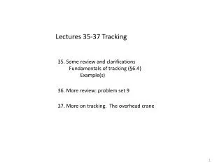
Lectures 35-37 Tracking. 35. Some review and clarifications Fundamentals of tracking (§6.4) Example(s ). 36. TBD. 37. More on tracking. The overhead crane. Lecture 35: Some review and clarification, and the essence of tracking. What does state space mean? What does T do?.

E N D
Lectures 35-37 Tracking 35. Some review and clarifications Fundamentals of tracking (§6.4) Example(s) 36. TBD 37. More on tracking. The overhead crane
Lecture 35: Some review and clarification, and the essence of tracking What does state space mean? What does T do? What are gains? What do we mean by tracking?
review The state vector describes the state of the system. Figuratively speaking, this tells us the position and velocity of every element The state equations then tell us how each element of the state evolves in time We can think of state space as having k “axes” that serve as a basis for the state vector The transformation between x and z spaces is simply a rotation of the sets of axes — the bases of the x and z systems The x and z vectors represent the same state viewed from different systems of axes That’s why the eigenvalues do not change
review Ax is a vector that points in some “direction” in state space bu is also a vector in state space The state vector changes in the direction indicated by the sum of these two vectors In order for the system to be controllable, we have to be able to make that vector point in any “direction”
review review The x space is given to us by the physics, and our choice of state vector We can find various z spaces to serve our purposes The diagonal transformation used the eigenvectors as a basis which is why we needed k independent eigenvectors for that to work The companion transformation has basis vectors in its T, which is where the controllability condition comes from (not obvious!) If we want x to be xr we need z to go to zr = Txr Bottom line: The state space is a way of representing the state of a system and we can pick what we like — limited by the physics!
review What are gains? We agree that we are using feedback control We feed back the output in an attempt to control it. The gains are the amount of each element of the state that we feed back. In the simplest case, where we have only a constant error, u = -gx They can be assembled in a row vector, which transforms when the coordinates transform which is why we have different gains in z space and x space
On to tracking The general idea We have a single input system and we want some reference state We can split x into two parts: the reference state and an error and then we can ask that e go to zero
The reference state is not totally arbitrary; it cannot be inconsistent with the physics. Friedland tackles the reference state and disturbances at the same time I’m going to tackle them separately, looking at tracking for the nonce We apply what we had on the previous slide:
We can ask what we really mean by tracking Do we really need to specify the whole state? Do we care about the whole state? For the magnetic suspension problem, we really only care about y For the overhead crane, we care mostly about y and to a lesser extent, about q So maybe all we need is to have part of the error go away?
In some cases we can find a ur to cancel the dynamics of the reference state We can do this if the problem is in companion form (although we may have some interpretation issues) We can often do it anyway (illustration to follow) But, we have to remember that we are finding the linear dynamics so, just as with basic control, we will have to verify our control in simulation
Companion form, tracking z1 = z1r We have z1 and we can find all the others one step at a time and when we get to the end, we can find ur We’ll be able to do this for the magnetic suspension problem without going to companion form
The problem From Kuo BC Automatic Control Systems yis positive down Numerical parameters for later
The coefficient c includes geometry, number of turns of the wire, permeability, etc There are many models of the force vs. gap equation none of them goes like 1/y An inverse square law is not a bad approximation, and I will use that as I did the last time we looked at this problem — we’ll be able to carry some stuff over As it happens, the behavior of the system, and its control, is qualitatively the same the same for any of the inverse models I will choose inverse square, and I will use the numerical coefficients given in Kuo (previous slide)
We have to linearize around a point other than zero We have a more complicated “Ohm’s Law” And we have a three dimensional state space
Manipulate the equations combine these input
Take a look at the equilibrium We require all the time derivatives to be zero From which we can express everything in terms of the equilibrium spacing
We can now set up the simulation and see how the equilibrium works We argued on physical grounds that it is unstable, and then we showed that it is unstable on mathematical grounds We make a simulation based on integrating the full equations of motion We denote the right hand side of the equations of motion by the vector F
The equations are nonlinear, so we need to linearize to deal with control To do that we use the equilibrium solution, which I found before
We want to linearize around the equilibrium solution This is the term that needs work I’ll deal with it on the next couple of slides
Let’s linearize using the “gradient” approach Think of expanding F in a three variable Taylor series around the equilibrium
Remember that So that the expressions become And these are the columns of the linearized matrix And we can get b by differentiating with respect to e
We have converted the original problem into a linear problem The eigenvalues of A are We see that the system is unstable which anyone who’s ever tried to do this will know
Suppose that we want to have the ball oscillate around its equilibrium position I don’t think I can do this using the nonlinear equations of motion We can do this in the linearized formulation. I want y = x1 to oscillate: y = dsin(wt) I don’t actually care about the other elements of the state but I certainly have to make the velocity the derivative of the position the current is not so clear, but it will have to be harmonic I have a linear problem, if some of it is harmonic, then the whole thing must be harmonic
Can I do this in x space, and can I cancel the entire xr piece? Let u = ur + u’
If I can get rid of all the extra terms, then I will have reduced the problem to the usual x —> 0 The third component will be harmonic, but it’s not clear what the phase is
We can use the differential equations to find a3 and b3 and ur
We know the problem is controllable, but let’s review that, too so it’s controllable
We want to use a gain matrix to stabilize this and then use to put it into the simulation, along with ur
We can look at simulations with the same poles that we used for the simple system We will find that the frequency of the oscillations is critical It works for low frequencies, but not for high Increasing the gain doesn’t seem to make much difference
Here’s where I’d like to stop and go to Mathematica to review and extend the magnetic suspension case The notebook goes like: Derive the general (nonlinear) equations of motion Build a simulation Linearize and design a linear control for equilibrium Test the control in simulation Choose a desired state and design a tracking control Combine the tracking and equilibrium controls and test in simulation