Download
1 / 14
140 likes | 166 Views
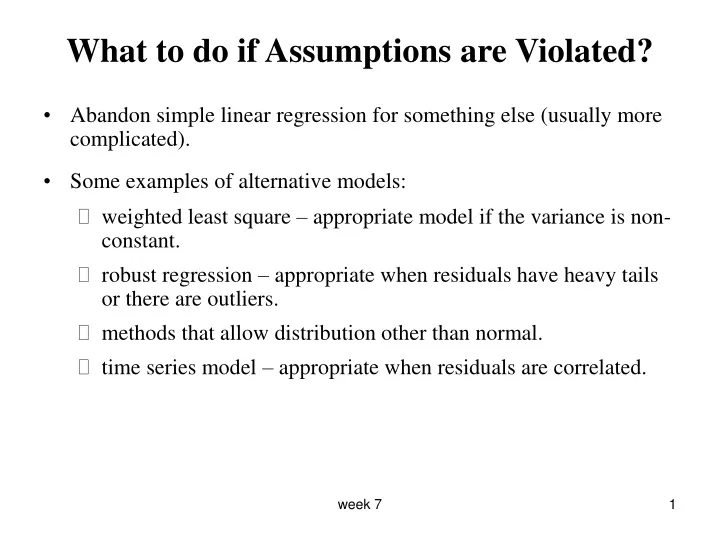
What to do if Assumptions are Violated?. Abandon simple linear regression for something else (usually more complicated). Some examples of alternative models: weighted least square – appropriate model if the variance is non-constant.

E N D
What to do if Assumptions are Violated? • Abandon simple linear regression for something else (usually more complicated). • Some examples of alternative models: • weighted least square – appropriate model if the variance is non-constant. • robust regression – appropriate when residuals have heavy tails or there are outliers. • methods that allow distribution other than normal. • time series model – appropriate when residuals are correlated. week 7
Dealing with Outliers / Influential points • First, check for clerical / measurement error. • Consider transformation if the points come from a skewed distribution. • Use robust regression which downplays role of extreme observations. • Consider reporting results with and without the outliers. • Think about whether an outlier is beyond the region where linear model holds; then fit the model on restricted rage of the independent variable. • For gross outliers that are probably mistakes, consider deleting them but be cautious if there is no evidence of mistake. week 7
Transformations • Transformations are used as a remedy for non-linearity, non- constant variance and non-normality. • If relationship is non-linear but variance of Y is approximately constant over X, try to find a transformation of X that results in a linear relationship. • Most common monotonic transformations are: • If curvature is non-monotonic then need a polynomial. This is done via multiple regression. • If the variance in non-constant, transform Y. week 7
More on Transformations • Very often we need to transform both X and Y. But… • Transforming X doesn’t change the distribution of the data about the regression line. It is equivalent to slicing the scatterplot into vertical slices and changing the spacing of the slices. • Transforming Y not only changes the shape of the regression line but alter the relative vertical spacing of the observations. • So transform Y first to achieve constant variance and then transform X to make relationship linear. week 7
Transformation to Stabilize the Variance • If Y has a distribution with mean and variance . Then the mean and variance of Z = f (Y) are approximately, • Proof: • This result gets used to derive variance stabilizing transformations. week 7
Examples week 7
SAS Example • In an industrial laboratory, under uniform conditions, batches of electrical insulating fluid were subjected to constant voltages until the insulating property of the fluids broke down. Seven different voltage levels, space 2 kV apart from 26 to 38 kV, were studied. • The measured responses were the times, in minutes, until breakdown. week 7
Interpreting log-transformed Data • If logY = β0 + β1X + ε then, . • The errors are multiplicative. • Increase in X of 1 unit is associated with a multiplicative change in Y by a factor of . • Example: • If Y = β0 + β1logX + ε, for each k-fold change in X, Y changes by β1logk. • Example: if X is cut in half, Y changes, on average by β1log(½). week 7
Violation of Normality of ε’s • By the Central Limit Theorem, linear combinations of random variables are approximately normally distributed, no matter what their original distribution is. • So CIs and tests for β0, β1, and E(Y) are robust (i.e., have approximately the correct coverage or approximately the correct P-value) against departures from normality as long as departures aren’t too extreme (outliers, skew). • Prediction Intervals are not robust against departure from Normality because they are for one point. week 7
Relative Importance of Assumptions • The most important assumption is independence of observations. There is no way around this with teachings from this course. • The second important assumption is the constant variance. Deviations from equal variance are OK if there is an equal number of observations at each value of X. • The least important assumption is Normality of the residuals, because of the CLT. It is, however, a necessary assumption for PI’s. week 7
More on Residuals • For all residual plots we use the raw residuals eias they are on the same scale as the response variable. • We can also use semi-studentized residuals which are defined as It is called “semi” because the MSE is an estimate of Var(εi) not Var(ei). • The semi-studentized residuals are useful for judging outliers; a point that is more than 3 S.D away from its mean is considered an outliers, i.e., if . week 7
Joint Estimation of β0 and β1 • A 95% CI for β0 capture the true value in 95% of possible samples. • A 95% CI for β1 capture the true value in 95% of possible samples. • But, the probability that both confidence intervals capture their true value is less then 0.95. • If we want to be 95% confident that both CIs capture their respective parameter, we can use a Bonferronie correction… • In general, for simultaneous CIs for any k parameters, the overall confidence level will be at least 100(1-α)% if the CI for each parameter is a 100(1-α/k)% CI. • These are called “joint” CIs, “simultaneous” CIs or “family” of CIs. week 7
Simultaneous Estimation of the Mean Response • We want to estimate CIs for the mean response E(Y) at more than one value of X simultaneously. • But the construction of CI is such that 95% of repetitions of sampling process result in intervals that include the correct mean response for that Xh. • If different 95% CIs are constructed for the mean response at more than one value of X, the proportion of repetitions in which the intervals include the true mean is less than 95%. • Again, we can correct for this by using Bonferronie correction; if we want simultaneous CI for k values of X, construct each CI at 100(1-α/k)%. • Alternatively, we can use the boundary values of the confidence band at selected X obtained from the Working-Hotelling procedure as simultaneous estimates of the mean response at this X. • Both of these procedures are conservative, i.e., the overall confidence level would actually be higher than 100(1-α)%. week 7
Inverse Prediction • Sometimes, a regression model of Y on X is used to make prediction of the value of X which gave rise to a new observation Y. • This is known as an inverse prediction. • We illustrate it with by an example (snow gauge)… week 7