Download
1 / 42
460 likes | 848 Views
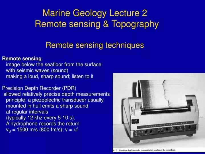
Marine Geology Lecture 2 Remote sensing & Topography Remote sensing techniques Remote sensing image below the seafloor from the surface with seismic waves (sound) making a loud, sharp sound; listen to it Precision Depth Recorder (PDR) allowed relatively precise depth measurements

E N D
Marine Geology Lecture 2 Remote sensing & Topography Remote sensing techniques Remote sensing image below the seafloor from the surface with seismic waves (sound) making a loud, sharp sound; listen to it Precision Depth Recorder (PDR) allowed relatively precise depth measurements principle: a piezoelectric transducer usually mounted in hull emits a sharp sound at regular intervals (typically 12 khz every 5-10 s). A hydrophone records the return vS = 1500 m/s (800 fm/s); v = f
major development in 1954 was the invention of the Precision Depth Recorder (PDR) at the Lamont Geological Observatory of Columbia University. This machine measured depths with errors of less than 1 percent of total water depth. The PDR discovered abyssal plains -- the flattest places on Earth. The PDR also helped Bruce Heezen, Marie Tharpe, and Maurice Ewing of Lamont discover the Mid-Atlantic Ridge Rift Valley in 1959. http://oceanexplorer.noaa.gov/history/electronic/1946_1970/electronic_middle.html Marie Tharp at Lamont, ca. 1961. "This picture is notable in its composition in that it shows the several factors of our work assembled in one place: original precision depth recorder (pdr) records are seen on the left-hand side other drawing board; on the upper right are seen the 6 original profiles plotted by Marie in 1952 which, correlated with deep soundings and shallow-focus earthquakes, led to the discovery of the world-encircling Rift Valley; Marie is shown working on her physiographic Diagram of the North Atlantic with crowquill pen and India ink, with the painted relief globe described elsewhere also on display.” http://www.earthinstitute.columbia.edu/library/Tharp/Bio1.html
side scan echo system: images "roughness" of bo"shadowgraph" projections from bottom yield enhanced echoes (dark areas) • eyes must adjust and consider illumination direction, • similar to stereo photos • Bottom towed (50 m off bottom) "fish" • downward looking 3.5 khz profiles • side scan system • Yields images similar to aerial photos; • Deep Tow system (SIO); • SeaMARC (Ryan, LDEO) • http://mp-www.nrl.navy.mil/marine_physics_branch/sidescan_deepwater.htm
Deep tow side scan echo http://woodshole.er.usgs.gov/project-pages/LakeMead/mapping.htm Lake Meade
Surface towed long-range sidescan system: GLORIAII towed at 50 m 6.2/6.8 khz sidescan w/30 s ping rate http://marine.usgs.gov/fact-sheets/seafloor/seafloor-4.gif
State of the art: Multibeam swath mapping: used by Navy for decades; declassified in early 1980's Seabeam 16 beams, swath width 0.75*water depth Hydrosweep 59 beams, swath width 1.8-2.0*water depth
Imaging below the seafloor • 12 khz echo sounding, max. 20 m penetration of bottom • 3.5 khz profiler, up to 100 m penetration Fig. 14 • used by Damuth to extensively map acoustic provinces related to sediment properties • slopes > 30°, poor return due to hyperbolae (bow tie artifacts) Fig. • to see sediments deeper than 100 m, need continuous seismic profiling • originally used explosives tossed off ship • now generally use higher frequency (better resolution, but less penetration) sound sources • f penetration • dynamite 4-60 10 • airgun 40-250 5 km • water gun 20-250 1-2 km • Sparker 60-500 1 km • transducer 3.5-40 kHz<50m • (fathometer) 40 khz 0 • human hearing 20 hz-20kHz
SCS Single Channel Seismic profiling (one or more hydrophones in one group/channel MCS Multichannel Seismic profiling (12, 24, 48, 96, or more channels (hydrophone groups)) principle is seismic reflection acoustic impedance (I) = density X velocity amplitude of reflection determined by reflectivity coefficient R = (v - v) / (v - v)e.g. V1 = 1.6 km/sec, V2 = 1.65 km/sec = 1.4 g/cc = 1.45 g/cc then R < 3% ( >97% energy is transmitted) Below: Lamont V3408 SCS profile http://rainbow.ldgo.columbia.edu/ees/data
REFRACTION (bending of waves) illustrate on board • Snell's Law - V1/V2 = sin Ø1/sinØ2 • i.e., large velocity contrast = large deflection • deflection can reach critical path along boundary • Seismic Refraction - measure velocity + thickness at single location based on achieving critical deflection according to Snell's Law • single source, many receivers spread out in line away from source
Magnetic Anomalies measured in (gammas) = 10-5 gauss Earth's field 65 k poles, 35 k equator measure at sea with proton precession magnetometer ("maggie") alternating current 20 khz, protons precess anomalies: measure as deviations from expected magnetic field (accounting for local variations in field) more northward oriented magnetized bodies below ship yield + anomaly; 100-1000 measure in sediments using spinner and cryogenic magnetometers Gravity mgal = 0.001 gal (cm/s2) Earth's field 980,000 mgal measure on ship to ±1.5 mgal correcting for ship's speed, course (Eotvos correction) height above sea-level & tides international gravity formula (due to flattening @ poles) Free air anomalies + over high submarine topography Simple Bouger correction: density correction Bouger anomaly: detect mass deficits e.g., the hot, less dense magma near ridge
Topography of the ocean floor Mean depth 3729 m; Greatest Depth = Challenger Deep - Marianas Trench (11000 m)
hypsometric curve: cumulative distribution of levels on Earths' surface two dominant physiographic provinces continents (0-500m elevation), ocean basins (mean depth 3800m) why? - reflects fundamental difference in density between ocean & continental crust why are they different? - chemical differentiation + erosion why do we have the end-members ?- very high and very low? -plate tectonics Ewing: brutal fact http://topex.ucsd.edu/es10/lectures/lecture06/hypsometry.gif
Matthew Fontaine Maury First contour map of the North Atlantic based on 200 lead weight soundings from aboard the Dolphin 1871-3 World Voyage of the HMS CHALLENGER Temperature readings revealed different temperatures on different sides of Mid-Atlantic Ridge http://www.earthinstitute.columbia.edu/library/TharpMapping.html
Heezen and Tharp physiographic maps - basic physiography, cartoon based on large but spotty PDR data set 1954 Precision Depth Recording Lamont scientist, Bernie Luskin, developed PDR to improve accuracy of deep sea soundings which led to improved mapping http://www.earthinstitute.columbia.edu/library/TharpMapping.html 1952 Six profiles based on soundings taken in the North Atlantic on cruises of Atlantis
1957 The first Heezen/Tharp Physiographic Map http://www.earthinstitute.columbia.edu/library/TharpMapping.html
Heirtzler/Edwards map - 1985 computer binned and generated bathymetric map; • one of first digital maps, done using conventional bathymetric (though digitial) data) • Sloss 1994 NOAA “Surface of the Earth” map based on geoid anomalies; • satellite altimetry data reflect minor variations in gravity due to topography • Sawyer 1995 - map also based on geoid anomalies, computer generated bath. • Smith and Sandwell (1997) the standard (NGDC [NOAA]) based on geoidal data • Visit http://www.ngdc.noaa.gov/mgg/image/global_topo_large.gif
Geoid - surface of equal gravity potential, dense things closer, surface moves up remove physical oceanographic (dynamic topography) and tectonic effects to obtain bathymetry (more assumptions, more detail, accuracy?)
4 oceans - have unique bathymetries PacificMAP, mean 3900m, surrounded by linear mountain chains, trenches, island arcs, marginal sea isolating deep basin from terrigenous input narrow continental margins large number volcanic island many marginal seas
Atlantic Ocean relatively long and sinuous, MOR in the center, prominent fracture zones linked to poles at N (Norwegian-Greenland Sea) and South as a result, different in deep circulation: NADW and AABW result, shorter residence time, more carbonate preservation greatest amount of freshwater discharge; more terrigenous sediments Where are Romanche Fracture Zone Charlie Gibbs Fracture Zone Bovet triple junction Scotian Arc Greenland-Scotland Ridge
Indian Ocean cross between A&P ridges are central (generally)some subduction zones, island arc (e.g., Indonesian arc)some long hotspot traces 90 E Ridgeabyssal plains & fans Largest microcontinent: Kerguelan Plateau
Arctic poorly defined (less data) MOR (Gakkel Ridge, ultralow spread rate) Aseismic ridge (Lomonsov) abyssal plains
Subbasins: • Atlantic: Norwegian, Greenland, Labrador, Newfoundland, North American, • Caribbean, Guiana, Brazil, Argentine, Weddell, Agulus, Cape, Angola, • Guinea, Cape Verde, Canary, Iberia, W Europe • Indian: Arabian, Somali, Mozambique, Masquerene, Crozet, Wilkes, • Australian, Wharton, Bengal • Pacific: Tasman, Bellingshausen, Scotia, Chile, Peru, Guantemala • marginal basins: South China Sea, Philippine, Japan Sea, • Okhotsk Sea, Bering Sea
Physiographic provinces: continental margins, ocean basins, and ocean ridges Margins continental shelfgradient <1:1000 (<0.05°); average width 78 km shelf/slope break ~135-200 m; generally subdued relief (< 20 m) effects of waves to 30 m slope >1:40 (>1.4°) 130-2000 m or so ("200-2000m); incised by v-shaped submarine canyons dominated by downslope processes (turbidity currents, mass flows) and hemipelagic rise more gentle (1:100) 100-100 km wide seaward thinning wedges of sediment mixture of downslope (turbidity currents, mass flows) & along slope (deep currents) processes and deposition canyons, channels cuts through
abyssal plains: flat. • typically 4-8 km; gradient <<1:1000; relief < 2 m • more common in Atlantic, Indian; few in Pacific - • why? rivers drain into Indian and Atlantic, • trenches trap seds in Pacific • even found at bases of trenches • seismic profiles show that they are thick accumulations of sediments • covering buried topography • made up of turbidites shed from continents: final resting place • abyssal hills <1000m 1-10km in width; occur in all oceans • Atlantic: generally between abyssal plains and MOR; common (?50%) • cover >80 % Pacific floor • basement features made of tholeiitic basalt; • excess volcanism near ridge crests • elongated parallel to axis of spreading • seamounts: >1000m relief; shield volcanos - accumulations of basalt lava flows - why basalt? • atolls formed on drowned seamounts (Darwin model) why drown? • guyots: flat topped seamounts: drowned atollsoften in linear chains (e.g., Hawaiian-Emporer system) • -why? PTT: trace of mantle hot spot
Mid-ocean ridges ≈ 2.5-3 km water depth (average 2.7 km) 80,000 km long MOR system (not really always MOR: e.g., EPR) often median rift valley: Atlantic slow spreading 1 cm/yr rate (1/2) Rift valley 1-2 km deep, few 10’s km wide Pacific faster spreading ridges; 5-10 cm/yr e.g., East Pacific Rise: no rift valley, less rugged topography basalt; visual obs. pillow lava Iceland: surface exposure http://video.google.com/videoplay?docid=-7255010558060211739
fracture zones fossil transform fault 10-100 km wide 100's to 3500 km long displace MOR changes in trends: reflect changes in direction of SFS
Ridge FZ FZ FZ Spreading direction change Transform fault Spreading direction change FZ Ridge
Trenches (topographic expression of subduction zone) • remarkably long and narrow < 100km wide, depths up to 11 km • Peru-Chile 5900 km long • ~ 1% Earth's surface • much more common in Pacific • only Puerto Rico, S. Sandwich in Atlantic • deepest part often filled with sediment
Oceanic rises = aseismic ridges • elevated portions of ocean floor not near continents or MOR • fairly gentle slope • origin; generally thermal anomalies/excess volcanism • Bermuda rise: 3000x1000 km upbowing of ocean floor • w/ 400-600 m total relief due to Eocene thermal anomaly (hot spot) • Darwin Rise: w/ Pacific: anomalous shallow large area attributed to mid-K volcanism; inlcudes Shatksy, Hess Rises (Pacific): great piles of volcanics • Ceara Rise, Rio Grande Rise • conjugate rises in S. Atlantic due to excess volcanism near ridge • 90E ridge: Indian Ocean; long linear feature, trace of hot spot • microcontinents: Rockall plateau: sits ~1000 m or so depth.; Aghulus P. off S Africa • Kerguelen P. Indian Ocean
Sunset over the Shatsky Rise, ODP Leg 198 The Vema today: the Windjammer cruise line’s Madalay
Homework: find these features on a map and determine their geological significance • Voring Plateau • Greenland-Scotland Ridge Denmark Straits, Iceland-Faeroe Ridg, Faeroe Bank Channel • Reykjanes Ridge • Charlie-Gibbs FZ • Rockall Plateau • SE Newfoundland Ridge • Sohm Abyssal Plain • Hatteras Abyssal Plain • Nares Abyssal Plain • Bermuda Rise • Puerto Rico Trench • Ceara Rise • Rio Grande Rise/Vema Channel • Romanche FZ • Walvis Ridge • Falklands/Malvinas Plateau • S. Sandwich Trench • Maude Rise • Aguhlus Plateau • Kerguelan Plateau • Broken Ridge • 90°E Ridge • Lord Howe Rise • Eltanin FZ • Ontong-Java Plateau • Shatsky Rise • Juan de Fuca Ridge • Clipperton FZ • Clarion FZ • Mendicino FZ • Emperor Seamount Chain • Hawaiian Islands • Kermadec-Tonga Trench • Mariana Trench • Japan Trench • Kuril Trench, Aleutian Trench • Bering Sea • Peru-Chile Trench