Download
1 / 23
230 likes | 461 Views
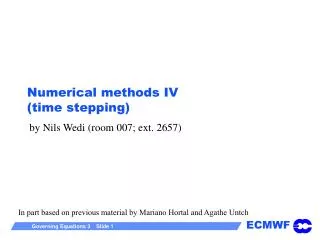
Numerical methods IV (time stepping). by Nils Wedi (room 007; ext. 2657). In part based on previous material by Mariano Hortal and Agathe Untch. What is the basis for a stable numerical implementation ?.

E N D
Numerical methods IV(time stepping) by Nils Wedi (room 007; ext. 2657) In part based on previous material by Mariano Hortal and Agathe Untch
What is the basis for a stable numerical implementation ? • A: Removal of fast - supposedly insignificant - external and/or internal acoustic modes (relaxed or eliminated), making use of infinite sound speed (cs) and/or the hydrostatic approximation from the governing equations BEFORE numerics is introduced. • B: Use of the full equations WITH a semi-implicit numerical framework, reducing the propagation speed (cs 0) of fast acoustic and buoyancy disturbances, retaining the slow convective-advective component (ideally) undistorted. • C:Split-explicit integration of the full equations, since explicit NOT practical (~100 times slower) Determines the choice of the numerical scheme
Choices for numerical implementation • Avoiding the solution of an elliptic equation fractional step methods (eg. split-explicit); Skamrock and Klemp (1992); Durran (1999) • Solving an elliptic equation Projection method; Durran (1999) Semi-implicit Durran (1999); Cullen et. al.(1994); Benard et al. (2004); Benard (2004); Benard et al. (2005) Preconditioned conjugate-residual solvers (eg. GMRES) or multigrid methods for solving the resulting Poisson or Helmholtz equations; Skamarock et. al. (1997); Saad (2003) Direct Methods; Martinsson (2009)
Split-explicit integration Skamarock and Klemp (1992); Durran (1999); Doms and Schättler (1999); ‘Slow’ part of solution ‘Fast’ part of solution e.g. implemented in popular limited-area models: Deutschland Modell, WRF model
Semi-implicit schemes linearised term, treated implicit (i) coefficients constant in time and horizontally (hydrostatic models Robert et al. (1972), Benard et al. (2004), Benard (2004) ECMWF/Arpege/Aladin NH) (ii) coefficients constant in time Thomas (1998); Qian, (1998); see references in Bénard (2004) (iii) non-constant coefficients Skamarock et. al. (1997),(UK Met Office NH model, EULAG model) non-linear term, treated explicit
Design of semi-implicit methods • Treat all terms involving the fastest propagation speeds implicitly (acoustic waves, gravity waves). • Assume that the energy in those components is negligible. • Consider the solvability of the resulting implicit system, which is typically an elliptic equation.
Example: Shallow water equations Linearized: Linear analytic solution: Phase speed: H denotes here a mean state depth.
Shallow water equations : advection : gravity-wave (or sometimes called ‘adjustment’) term In the linear version: advection adjustment combined In the atmosphere ==> Δt≤ 236 sec ~ 4 min in synoptic-scale models
x x x x x x x x x Explicit time-stepping • Leap-frog explicit scheme j+Δy j+Δx j-Δx j Stability: j-Δy If we treat implicitly the advection terms we do not get a Helmholtz equation
Increasing the allowed timestep • Forward-backward scheme forward backward doubles the leapfrog timestep von Neumann gives • Pressure averaging if ε=0 ------> leapfrog doubles the leapfrog timestep if ε=1/4 we get
Split-explicit time-stepping slow fast Stability as before but M times a simpler problem. Potential drawbacks: splitting errors, conservation. However recent advances for NH NWP suggested in (Klemp et. al. 2007) Note: The fast solution may be computed implicitly.
x x x x x x x x x Semi-implicit time-stepping j+Δy Solve: j+Δx j-Δx j j-Δy Helmholtz equation ! Stability: now onlylimited by the advection terms Note: if we also treat the advection terms implicitly we do not get a Helmholtz equation!
Compressible Euler equations Davies et al. (2003)
A semi-Lagrangian semi-implicit solution procedure (not as implemented, Davies et al. (2005) for details) Davies et al. (1998,2005)
A semi-Lagrangian semi-implicit solution procedure Non-constant- coefficient approach! Helmholtz equation (solutions see e.g. Skamarock et al. 1997, Smolarkiewicz et al. 2000)
Semi-implicit time integration in IFS Choice of which terms in RHS to treat implicitly is guided by the knowledge of which waves cause instability because they are too fast (violate the CFL condition) and need to be slowed down with an implicit treatment. In a hydrostatic model, fastest waves are horizontally propagating external gravity waves (long surface gravity waves), Lamb waves (acoustic wave not filtered out by the hydrostatic approximation) and long internal gravity waves. => implicit treatment of the adjustment terms. L= linearization of part of RHS (i.e. terms supporting the fast modes) => good chance of obtaining a system of equations in the variables at “+” that can be solved almost analytically in a spectral model.
For compact notation define: “semi-implicit correction term” Two-time-level semi-Lagrangian semi-implicit time integration in the hydrostatic IFS Notations: X : advected variable RHS: right-hand side of the equation L: part of RHS treated implicitly Superscripts: “0” indicates value at dep. point (t) “1/2” indicates value at mid-point (t+0.5Δt) “+” indicates value at arrival point (t+Δt) => L=RHS => implicit scheme L= part of RHS => semi-implicit (β=1) L=0 => explicit (β=0)
Semi-implicit time integration in IFS semi-implicit corrections semi-implicit equations
Semi-implicit time integration in IFS semi-implicit equations Reference state for linearization: ref. temperature ref. surf. pressure Where: => lin. geopotential for X=T => lin. energy conv. term for X=D
= unity operator Linear system to be solved Eliminate all variables to find also a Helmholtz equation for D+ : operator acting only on the vertical
One equation for each In spectral space (spherical harmonics space): because Semi-implicit time integration in IFS Vertically coupled set of Helmholtz equations. Coupling through Uncouple by transforming to the eigenspace of this matrix gamma (i.e. diagonalise gamma). Unity matrix “I” stays diagonal. => Once D+ has been computed, it is easy to compute the other variables at “+”.